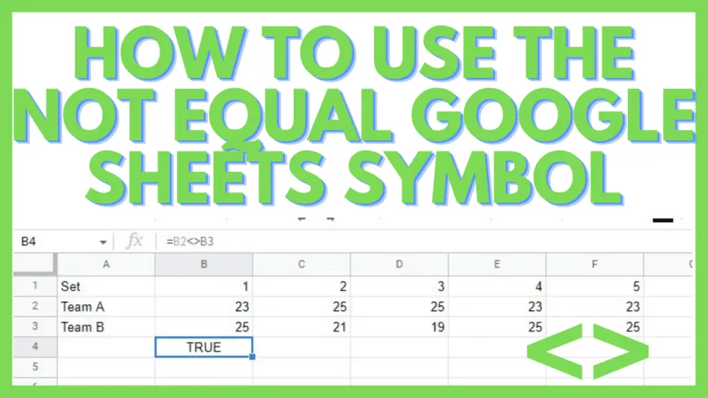
The Not Equal Google Sheets symbol in Google Sheets is “<>”.
Other than the more common comparative symbols such as the Equal To sign (=), the Greater Than sign (>), and the Less Than sign (<) – the lesser popular one is the Not Equal sign but it doesn’t mean that it is any less useful.
In this tutorial, I’m going to show you step by step how to use the Not Equal Google Sheets symbol in Google Sheets and other useful things about it.
The Not Equal To symbol, much like the other common logical operators, is best used in situations where you need to check run criteria checks.
How to Use the Not Equal Google Sheets Symbol
To use the Not Equal Google Sheets Symbol:
- Prepare the actual values or the references to two cells containing the values that you wish to compare
- Select the cell where you’ll want to input the formula
- Use this formula: “=value1<>value2”
How to Use the Not Equal Google Sheets Symbol <> Video Tutorial
The Common Uses of the Not Equal Symbol in Google Sheets
How to Use the Not Equal Google Sheets Symbol in Google Sheets To Compare Values
When doing so in Google Sheets, you use logical operators to get a boolean answer of either TRUE or FALSE.
This is highly valuable when you just need to identify if certain values in a dataset do not meet your required criteria.
In the example below, I’ve created a sample dataset and some conditions in columns D and E wherein if a person’s state and gender are not ‘Ohio’ and not ‘male’, respectively, their corresponding rows will return TRUE.

A good practice for this one is to select the cells where you expect your identifiers to be and go to Insert and select ‘Checkbox’.
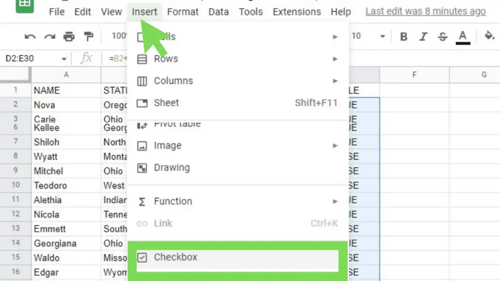
This will change the cells’ contents from being TRUE or FALSE to checkboxes where those that are ticked signify TRUE.

This way, it will be visually easier to see which among your dataset fits your criteria.
How to Use the Not Equal Google Sheets Symbol in Google Sheets For Conditional Formatting
By selecting the condition “Is not equal to” under the Format rules, I am able to simulate the same effect as when I’m using the Not Equal To symbol “<>”.
If you look at the example below, you can see that each highlighted cell in Column C corresponds to the ticked checkboxes in Column D.

Another way to do it via conditional formatting is through the ‘Custom formula’ option and directly inputting the formula similar to if you are typing it in regularly on the spreadsheet itself.
As you can see, the results are exactly the same as with the previous example where the Format rule “Is not equal to” was used.

Using the Not Equal function or symbol in Conditional Formatting helps a lot in presenting information in an easier-to-consume way.
You can learn more about Conditional Formatting by reading my previous tutorials about it.
You can also learn how to copy conditional formatting in Google Sheets.
IF-Condition Statements Using the Not Equal Google Sheets Symbol in Google Sheets
These functions require some logic to operate. That is why logical operators such as the Not Equal To symbol really shine when used with IF-condition statements.
The simplest IF-condition statement is
=IF(logical_expression, value_if_true, value_if_false)
=IF(logical_expression, value_if_true, value_if_false)
Here, you use the Not Equal To symbol in a statement and place it in the position of the ‘logical_expression’.
One great thing in using IF is that instead of just getting TRUE or FALSE as the results when you use a simple VAL1<>VAL2 statement, you can get modified values depending if the function returns TRUE or FALSE.
As you can see in the example below, I’ve added the IF statements on Column F. And if the value in Column B is not equal to “Ohio”, it will state “NOT OHIO”. Otherwise, if it is “Ohio”, then it will leave it blank.
 is working")
There are a lot more opportunities in using the Not Equal To sign in other IF statements such as COUNTIF, SUMIF, AVERAGEIF, and others.
If you want to get a better grasp of IF, you can check out one of my last tutorials about “if contains” formula here.
Other Ways of Using Not Equal Symbol in Google Sheets
Other than using the Not Equal sign (<>) in Google Sheets there is actually one more way to use the Not Equal logical operation which is through its functional equivalent.
Its function equivalent is
=NE(value1, value2)
=NE(value1, value2)
Where this function will check if ‘value1’ is NOT EQUAL TO ‘value2’. If they are not equal, this function will return TRUE, otherwise, it will return FALSE.
Writing the same thing using the sign gives us
=value1<>value2
=value1<>value2
This formula does the exact same thing as the previous one where ‘value1’ is being checked if it’s NOT EQUAL TO ‘value2’ and as such will return TRUE or FALSE depending on the validity of the actual values provided when the function is applied.
Recognizing opportunities when you can use the Not Equal To sign is an essential skill that everyone needs to learn especially if you always use spreadsheets on a regular basis.
Similar to how the more common logical operators like the equal to sign (=), the greater than sign (<), and the less than sign (>) are used, the Not Equal To (<>) is never any less important.
If to get to master all the logical operators in Google Sheets, it will be very easy for you to manipulate each and every function to get to your desired results.
This is one of the more basic functions that you need to master before you get to other functions such as the INDEX function.
Frequently Asked Questions On How to Use the Not Equal Google Sheets Symbol
Is Not Equal To “<>” in Google Sheets case-sensitive?
The Not Equal To sign doesn’t distinguish upper-case letters from lower-case ones. An alternative to this will be to use the EXACT function instead.
Can I use the Not Equal Google Sheets Symbol “<>” and the NE Function interchangeably?
The NE Function and the “<>” symbol work exactly the same way and differ only in syntax so you can use them interchangeably.
Conclusion On How to Use the Not Equal Google Sheets Symbol
To use the not equal Google Sheets symbol, prepare the two values that you wish to compare. Then select the cell where you’ll want to input the formula. Lastly, use this formula: “=value1<>value2”.

