You may have experienced trying to use variable cell references in Google Sheets whenever you have dynamic inputs but you just can’t figure out why it’s not working for you.
That is where the INDIRECT function in Google Sheets comes in.
In this tutorial, I am going to discuss how the INDIRECT function works in Google Sheets by using multiple examples.
Some practical uses of the INDIRECT function in Google Sheets are:
- To Lock a Cell Reference
- To Refer to a Cell in a different Sheet
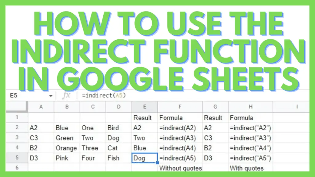
The INDIRECT function returns the cell reference specified by a string.
How to Use the Indirect Function in Google Sheets
To use the Indirect Function in Google Sheets:
- Choose the cell where you’re going to put the formula of the Indirect Function
- Prepare the cell_reference as a string or in a cell to be put into the formula
- If required, specify if your cell reference is on the A1 or R1C1 notation (optional)
- Type in the formula as “=INDIRECT(cell_reference_as_string, [is_A1_notation])”
Indirect Function in Google Sheets Video Tutorial
2 Best Ways To Indirect Function in Google Sheets
The INDIRECT function’s syntax is:
INDIRECT(cell_reference_as_string, [is_A1_notation])
The cell_reference_as_string parameter can be inputted with or without double quotes and each way has its own functionality. It can also be applied to ranges and named ranges.
1. Lock a Cell Reference Using the Indirect Function in Google Sheets
The INDIRECT function in Google Sheets gives us the capability to ‘lock’ specific cells relative to a formula.
This is impressive considering that typically, we can only lock rows or columns in Google Sheets.
For example, let’s take a look at the dataset below:

This is a list of diners who provide the highest discounts to locals from a certain city.
They are ranked from top to bottom with the highest discount-giving diners at the very top.
Since the discount rate of these diners changes from time to time, the top diner on the list changes as well – making it a dynamic list.

There were some formulas set that are affected whenever there are changes to the dynamic list of diners.
That said, it’s inconvenient that an update on the formulas needs to be done every time there’s a change to the list.

Whenever a diner gives out a higher discount, it is placed at the top of the list.

As you can see, when the list was updated and the cells were moved, the cell reference for cell E6 indicating the highest discount was automatically updated from ‘B2’ to ‘B3’.
Instead of showing the highest discount, it incorrectly displays the old-highest discount.
This requires you to update the formula to correct it. It is fine if it’s just a single list, but what happens if there are thousands?
This is where the INDIRECT function in Google Sheets comes in.
")
With the formula updated from a cell_reference (B2) to INDIRECT(“B2”), it should now be “locked” to display whatever value is in cell B2.

This is how you lock a cell reference using the INDIRECT function in Google Sheets.
2. Refer to a Cell in a Different Sheet Using the Indirect Function in Google Sheets
We’ve already touched on the possibility of having multiple lists with their own formula and the difficulties that can come with updating these formulas separately.
This time, we’re going to take a look at using the INDIRECT function to refer to different sheets at the same time.

In this example, we’ve taken a select list of 5 countries. We then created an ‘Overview’ page which will show the total population for their top 3 most populated cities. We used the following formula:
=Japan!B5
This will be done for each country in our sample list. Now, can you imagine if I listed all 195 countries in the world for this sample? It would definitely take a lot of time.

For this use-case scenario, we can use the INDIRECT function to write the formula:
=INDIRECT(B2&”!B5”)
This will come out as Japan!B5 which returns the value of the total population in its respective sheet (cell B5).
This can be inputted at the topmost cell in a range and you can just copy the rest until the bottom-most cell is filled out.

The cell_reference parameter for this example consists of both cell addresses with and without double quotes. The one with double quotes remained as itself while the one without returned the content of the cell it is referencing.
Common Errors with The INDIRECT Formula in Google Sheets
- Quotation marks around the cell reference parameter. B3 is different from “B3”.
- You may be putting invalid cell references depending on the notation that you’ve indicated as a parameter. Remember that TRUE indicates if the cell reference is in A1 notation or FALSE if it’s in R1C1 notation.
Frequently Asked Questions about Indirect Function in Google Sheets
Can I use the INDIRECT function in Google Sheets to return a value from a separate workbook?
You can use the INDIRECT function to recall values from other sheets in the same spreadsheet but not from an entirely separate workbook. An alternative to this will be to use the IMPORTRANGE function on a separate sheet and then use the INDIRECT function there.
Does the INDIRECT function in Google Sheets work on Named Ranges?
The INDIRECT function does work on Named Ranges. It can be done on the spreadsheet as part of a formula or it can be a part of the cell_reference section in the options of the Named Ranges menu.
Conclusion on Indirect Function in Google Sheets
To use the Indirect Function in Google Sheets you need to choose the cell where you’re going to put the formula of the Indirect Function and prepare the cell_reference as a string or in a cell to be put into the formula. If needed, specify if your cell reference is on the A1 or R1C1 notation then type in the formula as “=INDIRECT(cell_reference_as_string, [is_A1_notation])”

