How to Use the Index Function in Google Sheets – #1 Tutorial

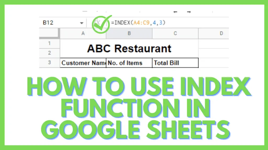
In this tutorial, I am going to guide you on how to use the Index Function in Google Sheets.

For this, first, let’s see what the index function is used for. in Google Sheets. An Index Function is used to look up and return/extract the information from the selected range of cells.

The function uses an entire range, also called the input range, which is specified by the offset based on column and row so that it can locate the cell and displays the content in the given area (the cell in which you applied the function).

This function can be combined with other functions and the results are astonishing because they help a lot in maintaining and organizing huge amounts of data that seem impossible to be arranged.

A perfect example of this combination of two functions can be The Index and Match Function.

Index Function in Google Sheets

To use the Index Function in Google Sheets:

1. Select the Range (reference)
2. Add the Row (Number) to the Function
3. Add the Column (Number) to the Function
4. The Index Function is Applied

How to Use the Index Function in Google Sheets Video Tutorial (Step-By-Step)

Syntax of the Index Function in Google Sheets

For a better understanding, let’s have a look at the syntax of the index function to make it clear to you.

The syntax for the index function is:

INDEX (reference, [row], [column])

Here, as you can see, the above function has 3 parameters:

• reference
• row (optional)
• column (optional)

Reference

Soon as you apply the index function the first thing that Google Sheets demands from you to select is the Reference.

Reference is the Range of the cells that you are supposed to select and from which your data will be extracted. You may also call it the Input Range.

Now, it is very clear that you should select your entire table that contains your data (if applying the function on the whole Sheet) because if you skip any of your rows or column then the index function would not consider that row and column and there are chances that you may make an error in your spreadsheet.

Row (optional)

After selecting the reference (input range) the next thing that you will come across is the row.

The row is that specific Row Number from which you want to extract your data. The main thing to be considered here is that the row number should be within the range of cells that you have selected.

Column (optional)

The last thing in the index function to put on is the column. Column here means the specific Column Number from which you want your data to be extracted.

And again, the important thing to be considered here (and in a row also) is that the column you are selecting should be within the reference or range you had selected first.

Note: Only the reference parameter is the mandator for the index function. The row and column parameters are optional. If you do not provide the last two, the whole data table that you selected will be extracted.

Also, if your Row number and Column number are out of the reference then an error will occur.

How to Use Index Function in Google Sheets – Step-by-Step

Now let me solve an example in front of you where we will apply the index function. Here is a step-by-step guide.

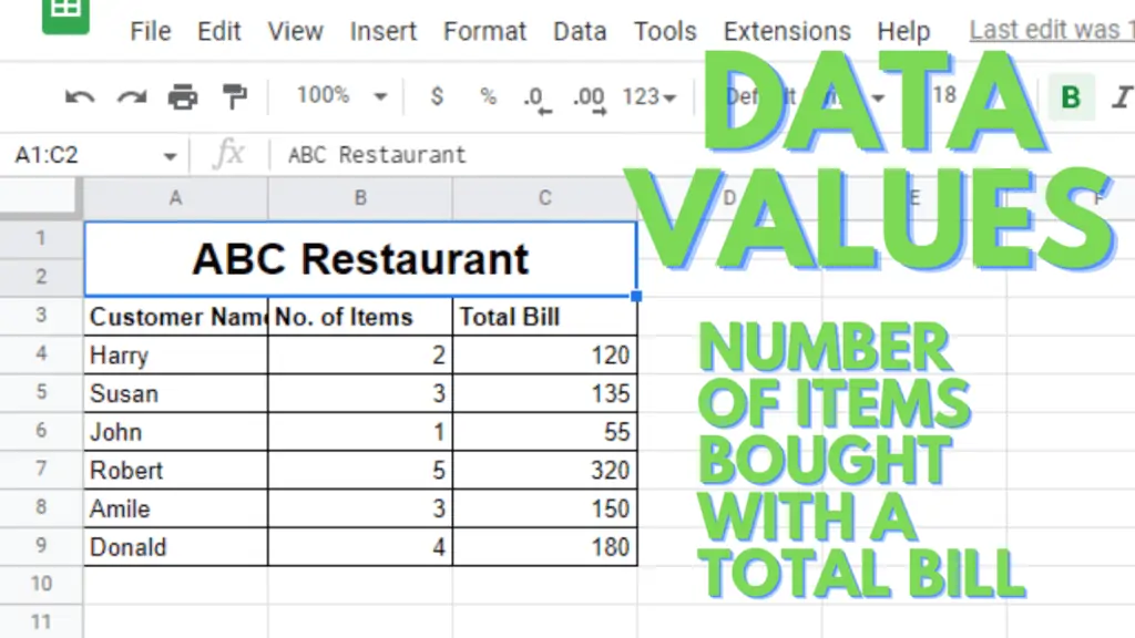
So, first of all, let’s take a dataset to apply the index function to it. Here, we are taking an example of a small restaurant at which customers arrive and they have an order of different items say burger, fries, hotdogs, drinks, etc.

In this, we will be having the dataset of 6 customers that order some items and at last, we will be having their total bill.

Step 1 – Select the Range (reference)

Let’s just say we want to extract the total bill of our 4^th customer Robert. For this, first of all, for using the index function (or even any other function/formula in Google Sheets):

1. Select the cell, where you want to apply the function/formula
2. Press Equal “=”. This will initiate the calculations.
3. Write =Index in the cell. Google Sheets will show you the suggestions as you type.
4. Keeping the Index function active in the suggested list, double-click on it using your mouse or press “Tab” from the keyboard.
5. The Index function is initiated.

Now, our first step will be selecting the range as our reference for the application of the index function. In our above example, we will be selecting our entire table as the reference except for the header row.

So, in this case, our reference or you may say the input range will be A4:C9.

Step 2 – Adding the Row (Number) in the Function

Just after selecting our reference for the index function, the next step is to define from which row you want your specific data to be selected.

As we have decided above, we want the data of our 4^th customer Robert who is in the 4^th row of our selected data reference so our row number will be 4 here.

Note: If you want the data of any other customer then you need to change the row number accordingly.

Step 3 – Adding the Column (Number) in the Function

The last and final part of the index function is to specify the column number. In the above example, as we can see that the Total Bill is displayed in the 3^rd column so the column number in the function will be 3.

Note: Similar to this case, if you want any other data about the customer then you need to change the column number accordingly۔

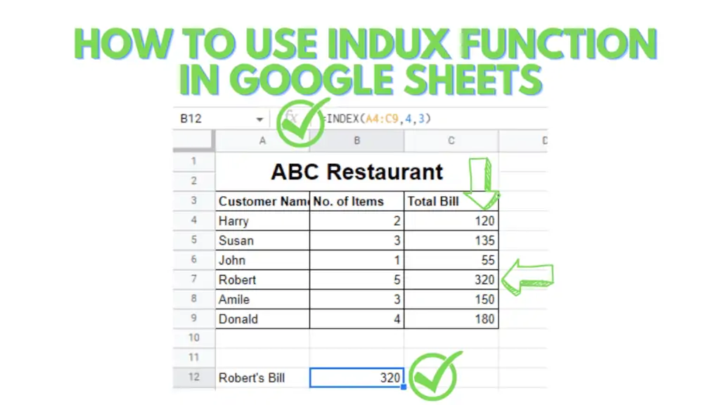
Step 4 – Index Function is Applied

As soon as you are done with the above three steps you will be having your complete function in your cell. Make sure that if you are following my example then your index function should be like this:

=INDEX(A4:C9,4,3)

Now the only thing left is to press Enter key and you are done.

Conclusion On How to Use the Index Function in Google Sheets

To use the index function in Google Sheets put the reference (data table/range), row number (optional) & column number (optional) into the formula INDEX (reference, [row], [column]) to extract any cells or information from the selected data table/range.