The Index and Match Functions in Google Sheets

Individually, the INDEX Function or the MATCH Function are simple to use but their application is limited. When used together, they become way more powerful.

In this tutorial, I am going to show you how to use the INDEX and MATCH Functions in Google Sheets.

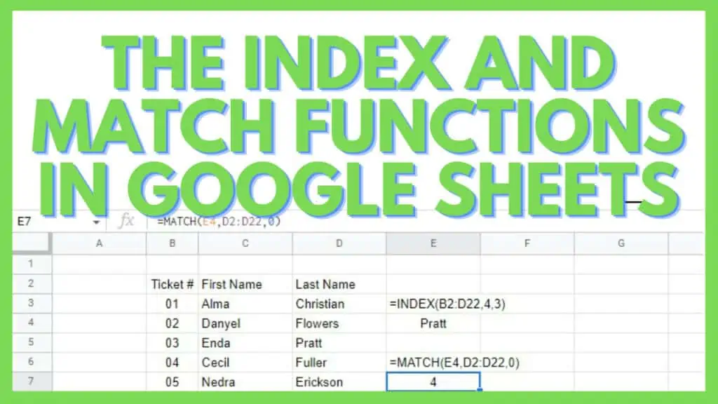
How to Use the Index and Match Functions in Google Sheets

1. Determine the range1 where the result will be taken from
2. Identify range2 which will be the reference for the value to be returned
3. Define the search_key parameter
4. Use this formula: =INDEX(range1,MATCH(search_key,range2),0))

Using the Index and Match Function in Google Sheets Video Tutorial

Using the INDEX Function

In the first part of the INDEX and MATCH Functions in Google Sheets, INDEX returns the content of a cell, specified by row and column offset – but in our case, is specified by the output of MATCH which I’m going to explain later.

The syntax of INDEX is:

=INDEX(reference, [row], [column])

Where

• Reference – the range where the leftmost column has a row and a column value of 1
• Row – the row value respective to the reference parameter
• Column – the column value respective to the reference parameter

I recreated the multiplication table for the example below. Assigning the whole table as the reference (C4:K12), 5 as the row parameter, and 6 as the column parameter produces 30 as its result.

The topmost row and leftmost column contain the basic numbers 1-9 which also matches the row and column respective to the reference for this selection.

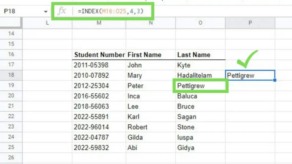
I’ve created another example with a simple table containing student numbers and student names.

This time, I’ve assigned the whole table with its headers included as the reference. The top leftmost value which is ‘Student Number’ has the coordinates (1, 1).

I have also assigned the value 4 for the row parameter and 3 for the column parameter for the INDEX Function.

Counting 4 down and 3 right gives me “Pettigrew” as seen below.

The use of the INDEX Function is indeed limited but is extremely powerful as a feature if combined with the next part of the tutorial, the MATCH Function.

Using the MATCH Function

The second part of the INDEX and MATCH Functions in Google Sheets, MATCH returns the relative position of an item in a one-dimensional range that matches a specified value – which in our case acts as the row or column value of the INDEX Function.

The syntax of MATCH is

=MATCH(search_key, range, [search_type])

Where

• Search_key – the value to be searched
• Range – the one-dimensional array to be searched
• Search_type – optional and can be 1, 0, or -1 (I suggest that you use 0 for an exact match – otherwise 1 will be for “ascending-highest” while -1 will be “descending-smallest”)

I’m using the multiplication table again as an example for the MATCH Function this time.

Now, instead of using “coordinate” to get the value in this table, I’m doing the inverse of that where I’ll be searching for a value in a certain row or column, and I’ll be getting one of its factors.

In the example below, I’m looking for the value ‘24’ on the row for ‘8’ which is J4:J12. In other words, I’m looking for a factor of ‘24’ other than 8, and this gives us the number ‘3’ – in the context of MATCH, this is the position of ‘24’ in the range J4:J12 where J4 is ‘1’.

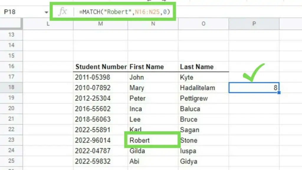
Using again the same table as earlier and doing the inverse for the MATCH Function as well, I’m looking for the First Name “Robert” on the First Name column.

In doing so, I got the result ‘8’ which is the position of “Robert” in the range N16:N25 where N16 is ‘1’.

MATCH is often useful if you’re looking for a specific item in a large dataset or when you’re trying to define the row or column of said item in that large dataset.

Other than this, it’s best used in tandem with the INDEX Function which I’m going to show in the next part of this tutorial below.

Using the Index and Match Functions in Google Sheets

Before we start with the main topic of this tutorial, I would like to touch on the VLOOKUP Function first which works as something that searches down the first column of a range for a key and returns the value of a specified cell in the row found.

The syntax of VLOOKUP is

=VLOOKUP(search_key, range, index, [is_sorted])

It works similarly to the INDEX and MATCH Functions in Google Sheets but there is a limitation that I would like to show below.

For my first example, I used it normally and set the whole table below as the range with ‘14’ as the search_key.

Using a table with three columns like this automatically assigns an ‘index’ value to each column where the left-most column is ‘1’, the next is ‘2’, and in our case, the last is ‘3’.

The ‘index’ that I’ve selected is ‘3’ because I need to look for the Last Name associated with Ticket # ‘14’.

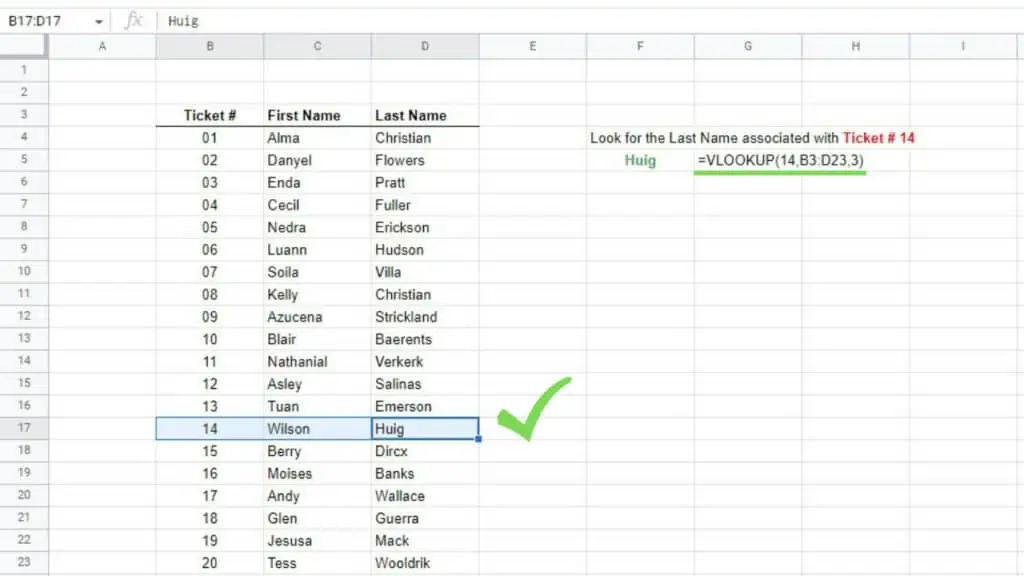
This gives us the answer as ‘Huig’.

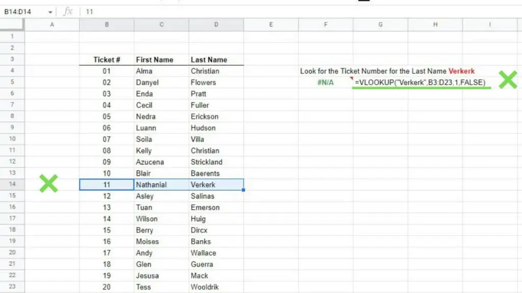
In my second example for VLOOKUP, a problem happens. Using the same table, with the search_key “Verkerk” which is the last name, the error comes from the fact that the search_key must be in the first column of the selected range which will be “Index 1”.

Unfortunately, in this example, the “Last Name” column is on the last one and when we try to use VLOOKUP in this situation we get an error.

This is where the INDEX and MATCH Functions in Google Sheets shine the best.

Unlike VLOOKUP, INDEX MATCH can work even if your search_key is at the rightmost column of your table or dataset.

The formula for the INDEX MATCH is

=INDEX(range1,MATCH(search_key,range2),0))

Where:

• Range1 – the row or column from which INDEX takes the final output
• Range2 – the row or column where the search_key will be checked against to determine the reference position for INDEX
• Search_key – the value or string to be searched in MATCH

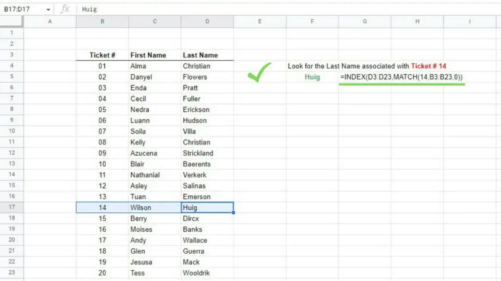
Applying the INDEX MATCH below in the same settings as the first example of VLOOKUP gives us the same correct answer which is ‘Huig’.

Now, I’m going to use INDEX MATCH to the same example as the 2nd one in VLOOKUP where we encountered an error.

I’ve used the formula: “=INDEX(B3:B23,MATCH(“Verkerk”,D3:D23,0))” where the main difference compared to VLOOKUP is that instead of selecting the whole table as the range, I’ve assigned the two individual columns to range1 and range2 differently.

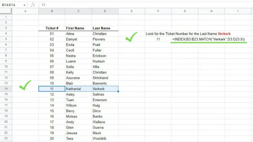
As you can see, it worked and we got the answer that the Ticket # with the Last Name “Verkerk” is ‘11’.

Using INDEX MATCH in Lieu of HLOOKUP

For my last examples, I’ve used the INDEX and MATCH Functions in Google Sheets in lieu of the VLOOKUP Function.

That said, it can also be used with the HLOOKUP Function and the only difference is that for the former, the search goes vertically in columns while the latter goes horizontally in rows.

The syntax of HLOOKUP is

=HLOOKUP(search_key, range, index, [is_sorted])

Where the parameters are the same as those of VLOOKUP, but they should be looked at horizontally this time.

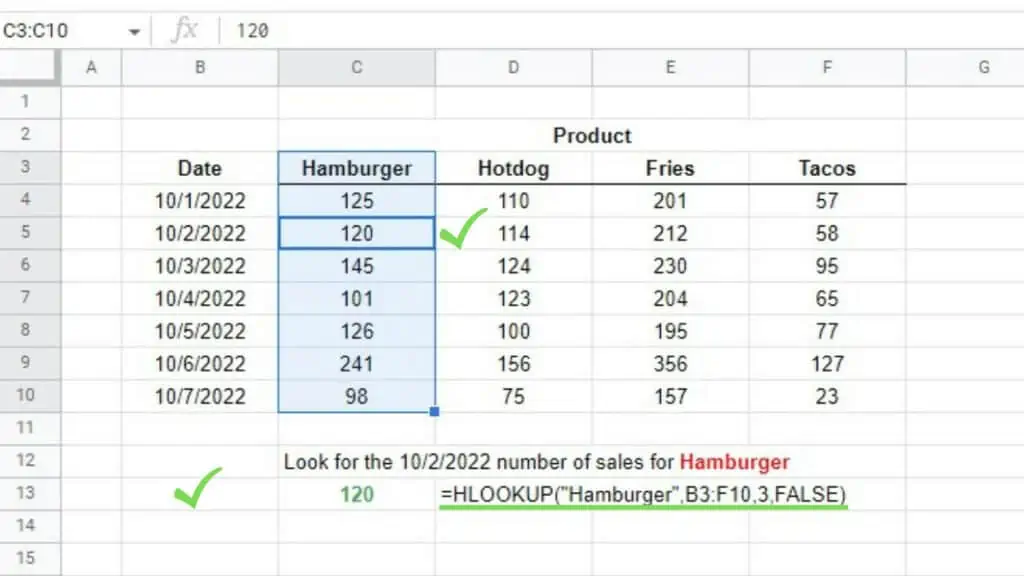
Again, similar to VLOOKUP, I applied HLOOKUP to the example below where the index row is at the very top or the first position on the selected range.

In doing so, we get the answer that the Hamburger sales last 10/2/2022 is 120.

Now, the issue with VLOOKUP is when the index column of HLOOKUP is not at the top or first position but instead is at the middle like this one below.

I wanted to know which product is the highest selling product last 10/4/2022 so I used max for that date and that became my search_key. Unfortunately, that date is in the middle of the range and is below the desired answer which is ‘Fries’.

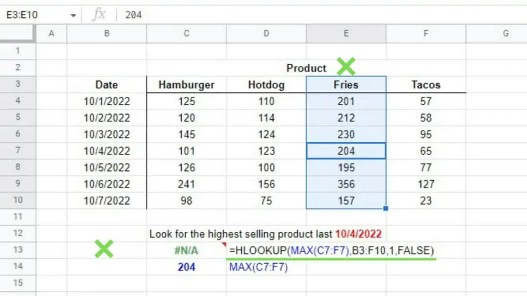
Pushing for the HLOOKUP formula in this case results in an error.

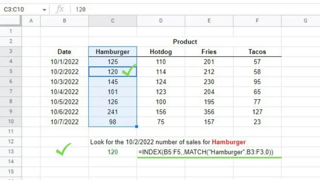
Just like before, we can instead use the INDEX and MATCH Functions in Google Sheets.

For the first example, the INDEX MATCH formula gives us the same answer as HLOOKUP.

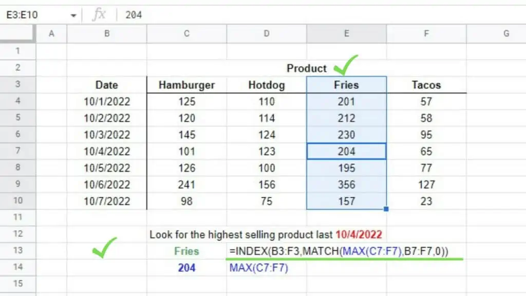
For the next example where we encountered an error, I used the formula: “=INDEX(B3:F3,,MATCH(MAX(C7:F7),B7:F7,0))” where the MATCH Function acted as the column value for the INDEX Function.

In doing so, I was able to determine that the highest selling product last 10/4/2022 was ‘Fries’!

The INDEX and MATCH Functions in Google Sheets may not be as simple to understand at first but is incredibly rewarding once you do.

This unlocks different ways to do things especially if you are hindered by scenarios where you can’t use the favorites VLOOKUP and HLOOKUP.

Frequently Asked Questions about The Index and Match Functions in Google Sheets

Conclusion On Using The Index and Match Functions in Google Sheets

Use the Index and Match Functions in Google Sheets by determining the range1 parameter where the result will be taken from and the range2 parameter which will be the reference for the value to be returned. Next, define the search_key parameter and then use this formula: “=INDEX(range1,MATCH(search_key,range2),0))”.