In this tutorial, I’m going to show you how to use the IF function in Google Sheets.
I often use Google Sheets as a powerful calculator or as a free database but I also use it as a tool that helps me in scenarios where decision-making is needed. This is done by using the IF function.
IF allows you to check certain values or functions and give you the option to have a value depending on whether your conditions were met. I use the IF function in Google Sheets often and have mastered its basics – so if you’re having a hard time using it let me share this tutorial with you.
How to Use the IF Function in Google Sheets
- Determine the logical expression for your IF-condition statement
- Define the value-to-be if your statement is true
- Likewise, specify the value-to-be if your statement is false
- Use this formula: “IF(logical_expression, value_if_true, value_if_false)”

IF Function in Google Sheets Video
The Syntax and the Logical Expression for the IF Function in Google Sheets
The IF Function has a straightforward syntax but depending on how you need or use it, it can also be complex to produce more accurate results.
The syntax of IF:
=IF(logical_expression, value_if_true, value_if_false)
For the logical_expression parameter, you can compare two cells, values, or functions with the operators below:
| > | greater than |
| >= | equal to or greater than |
| < | less than |
| <= | equal to or less than |
| <> | not equal to |
| = | equal to |
As for the parameters ‘value_if_true’ or ‘value_if_false’ – these can be values, references to cells containing the values, or even formulas that you wish to be returned whether the logical expression/criteria is met (TRUE) or not (FALSE).
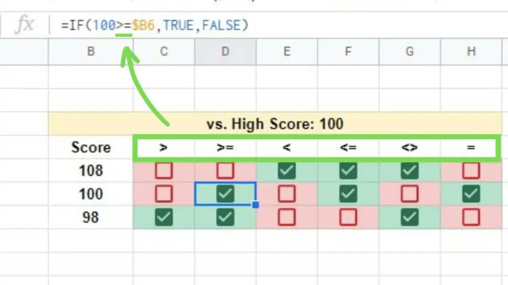
I created a chart below visualizing how each logical operator works with the value 100 when compared to the values 108, 100, and 98.
A checked box represents TRUE (Green) while an empty box represents FALSE (Red).
Taking a few examples below this means that:
- 100 > 108 → FALSE
- 100 >= 100 → TRUE
- 100 < 98 → FALSE
- 100 <= 108 → TRUE
- 100 <> 100 → FALSE
- 100 = 98 → FALSE
Depending on what your needs are, you may use these operators alone or in combination with one another.
4 Basic Uses of the IF Function in Google Sheets
I’m going to show you how to use the IF Function in Google Sheets in 4 different ways.
1. Basic Use of the IF Function for Only Two Possible Results
The basic purpose of the IF Function in Google Sheets is to present you with two options if your condition is met or not.
This is the basic use of IF, strictly adhering to its syntax.
In the example below, I’ve created a dataset wherein a student’s average between two exams is calculated and if the student gets a score of 75 or higher, the student passes.
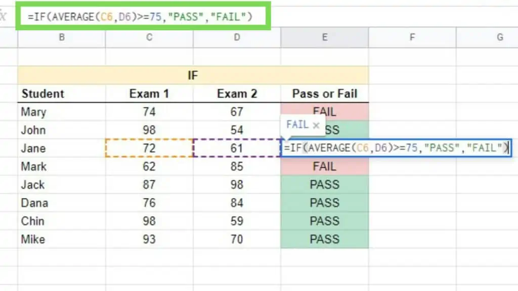
As you can see, I’ve directly inputted the AVERAGE Function as part of the logical_expression parameter. Together with the >= (greater than or equal to) operator, it is compared to the static value of 7, which is the passing score for this example.
2. AND Function for Multiple Condition Checks (All)
Similar to my prior example, I’ve shown you how it is possible to have other functions or formulas in the logical_expression parameter. That said, that example only shows one condition where the student’s average score must be equal to or greater than 75.
For this method, I’ll be using the AND Function.
In the example below, I have two conditions that must be BOTH true for IF to return the value_if_true parameter (which in this case is TRUE).
Basically, if a student has perfect attendance and a final rating greater than 95, that student will be part of the “Honor Roll”.
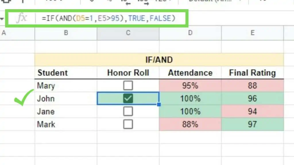
As you can see, only John met both conditions where he achieved both a perfect attendance of 100% plus a final rating of 96.
The AND Function strictly checks both conditions if they are TRUE before it returns TRUE. Otherwise, it will return FALSE.
3. OR Function for Multiple Condition Checks (One or Some)
This time, I’ll be using the OR Function.
I’ve modified the previous example. Instead of checking for students that will be part of the “Honor Roll”, I will be checking for students that will be part of the “Recognition” program.
The qualifications for a student to be part of the “Recognition” program is that the student must either get perfect attendance or must get a final rating greater than 95.
The OR Function checks if EITHER or BOTH conditions are TRUE and if so, will return TRUE. Only if both conditions are FALSE will it return FALSE – as seen in the example below.
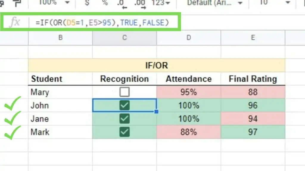
With this example, John, Jane, and Mark will all be part of the “Recognition” program even though they each passed differently.
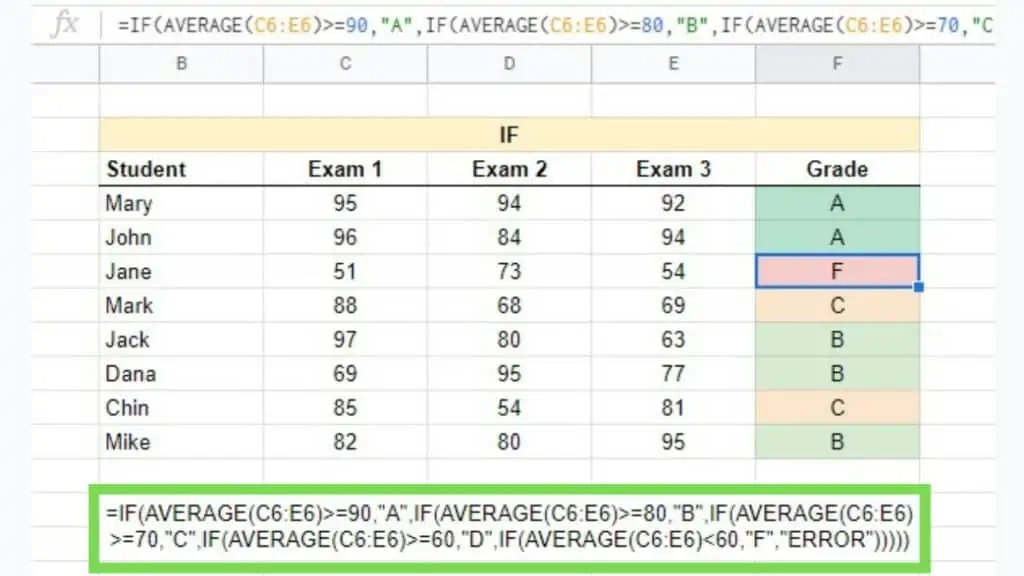
4. Nested IF Function for Multiple Result Possibilities
I’ve been discussing mostly how the logical_expression parameter of the IF Function in Google Sheets can be utilized best. In this method, I’ll show you how to use the IF Function as part of the value_if_false parameter to allow for multiple result possibilities.
In its most straightforward usage, IF only outputs two possible values depending if the condition is TRUE or FALSE. But I’ve also mentioned that you can use formulas as the value-output which includes the IF Function.
The basic syntax allows for two options, but to have three more options the syntax will be:
=IF(logical_expression, value_if_true, IF(logical_expression, value_if_true, value_if_false))
To add more options, just change the last ‘value_if_false’ to another IF Function and so on.
In the example below, I created a simple rubric for what the grade equivalent of students will have depending on their average score for exams one, two, and three.
- A: Average >= 90
- B: Average >= 80
- C: Average >= 70
- D: Average >= 60
- F: Average < 60
- ERROR (for non-numerical values)
To do this, nested four (4) more IF Functions inside one IF giving me 5 IFs with 6 options in total.
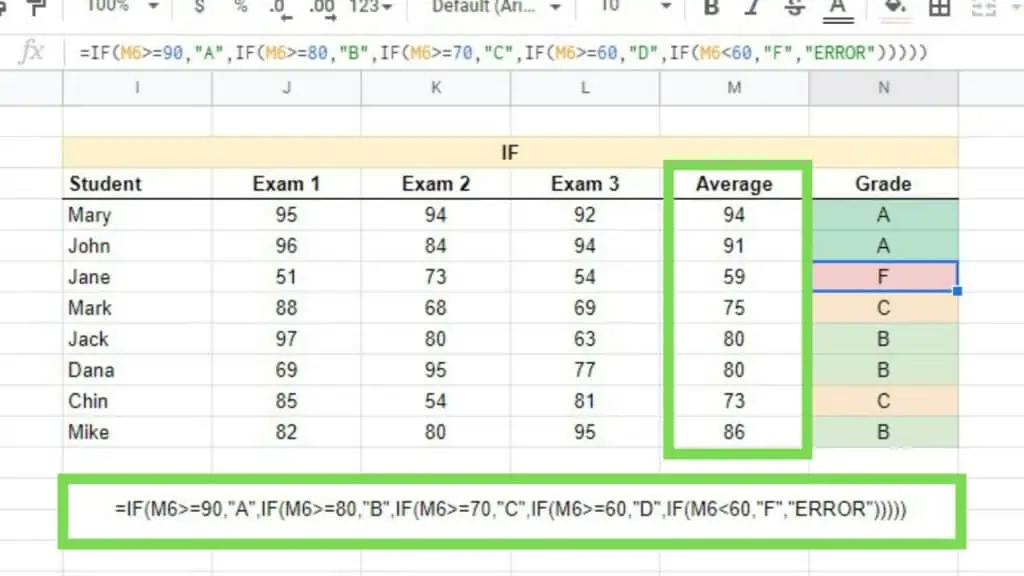
In the previous example, since nesting more IF Functions in Google Sheets required me to put a logical expression for each IF, I ended up with a very long formula.
To avoid this, I simply created an extra column where the average is and used it as a reference for the logical_expression parameter.
Take note that IF can also be used to check for comparison in dates and strings.
Other than using the regular logical expressions for the IF Function in Google Sheets, there is also a way to check if a cell or string contains something specific that you are looking for.
If you are interested, check my previous article to know the Google Sheets formula for IF Contains.
Frequently Asked Questions about How to Use the IF Function in Google Sheets
How can I use logical expressions with texts in the IF Function in Google Sheets?
You can use texts as the values to be compared with operators in the IF Function in Google Sheets by enclosing the string in double-quotes. If you want to check for the double-quotes character, use the function CHAR with the value “34” → CHAR(34).
How can I use logical expressions with dates in the IF Function in Google Sheets?
You can use dates as the values to be compared with operators in the IF Function in Google Sheets by treating them the same as regular numbers. You must make sure that each date is recognized by Google Sheets as a date value, to check this use the DATEVALUE function.
Conclusion on How to Use the IF Function in Google Sheets
To use the IF function in Google Sheets by determining your IF-condition statement’s logical expression first and then defining the value-to-be if your statement is true. Likewise, specify the value-to-be if your statement is false and lastly, use this formula: “IF(logical_expression, value_if_true, value_if_false)”.

