How to Wrap Text in Google Sheets

In this tutorial, I will show you how to wrap text in Google Sheets.

Text wrapping allows you to set rules on whether to automatically resize a cell or certain columns or rows, have it overflow to the unfilled columns, or clip its display, a useful tool in maximizing limited display space in Google Sheets.

Select a cell or range
Click on Format from the Menu Bar
Highlight Wrapping from the Format Menu
Select a Wrapping option between Overflow, Wrap, or Clip

Wrap Text in Google Sheets YouTube Tutorial Video

Text Wrapping in Google Sheets Options Explained

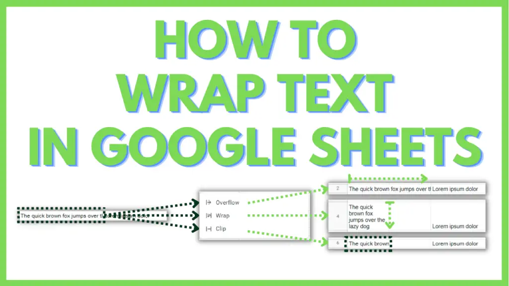
wrapping: formatting setting that dictates how the cell will behave when its contents exceed the cell dimensions
overflow: type of wrapping that allows the cell to overflow its contents to succeeding empty columns. The default wrapping for all cells.
wrap: type of wrapping that allows the cell to automatically increase its row height to display as much of its contents as possible
clip: type of wrapping that restricts the display of a cell’s contents to within its dimensions only

Wrap Text in Google Sheets Step by Step

For this tutorial, I will provide a sample file that will have 1 worksheet. This worksheet is a grid of text, organized across 3 columns in a way where we can demonstrate how text wrapping works in certain situations.

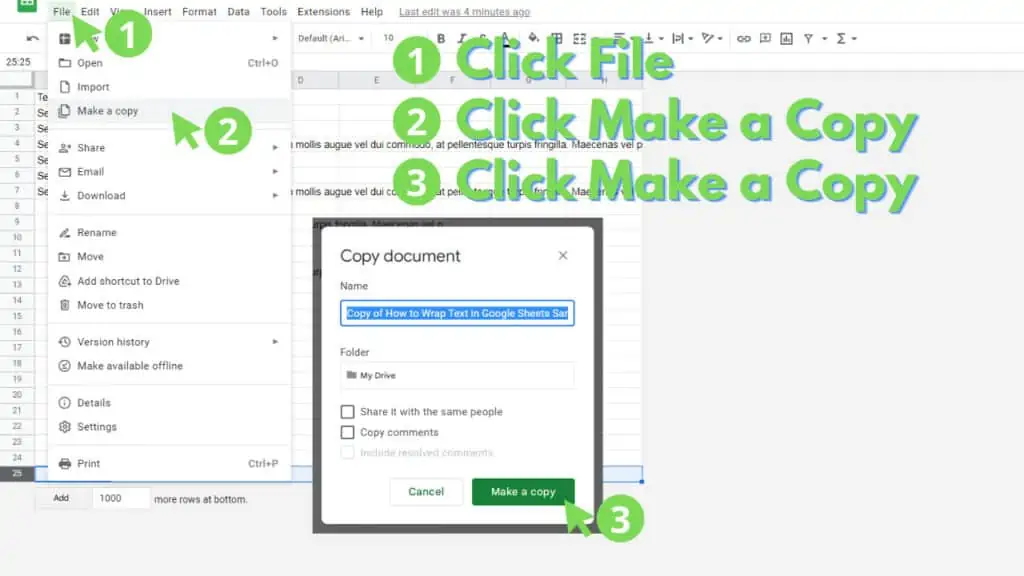
You can make a copy of the file by accessing it through this link, then by clicking on “File” from the menu bar, then by clicking on “Make a copy”.

A dialog box should appear. Within it, you can provide a filename for the copy then click “Make a Copy”.

Step 1 – Select a cell or range

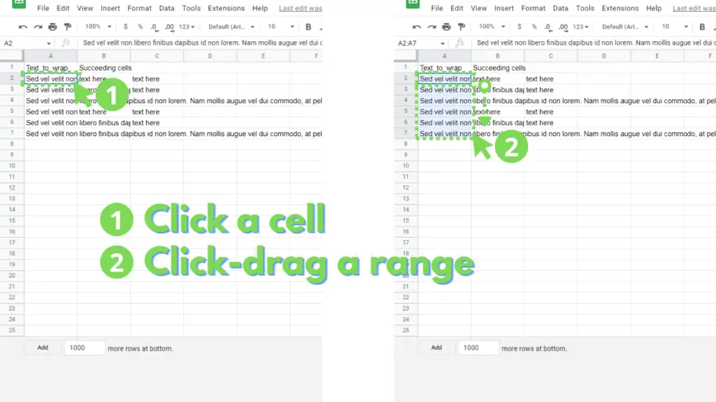
The first step in wrapping text in Google Sheets is to select a cell or range to apply wrapping to.

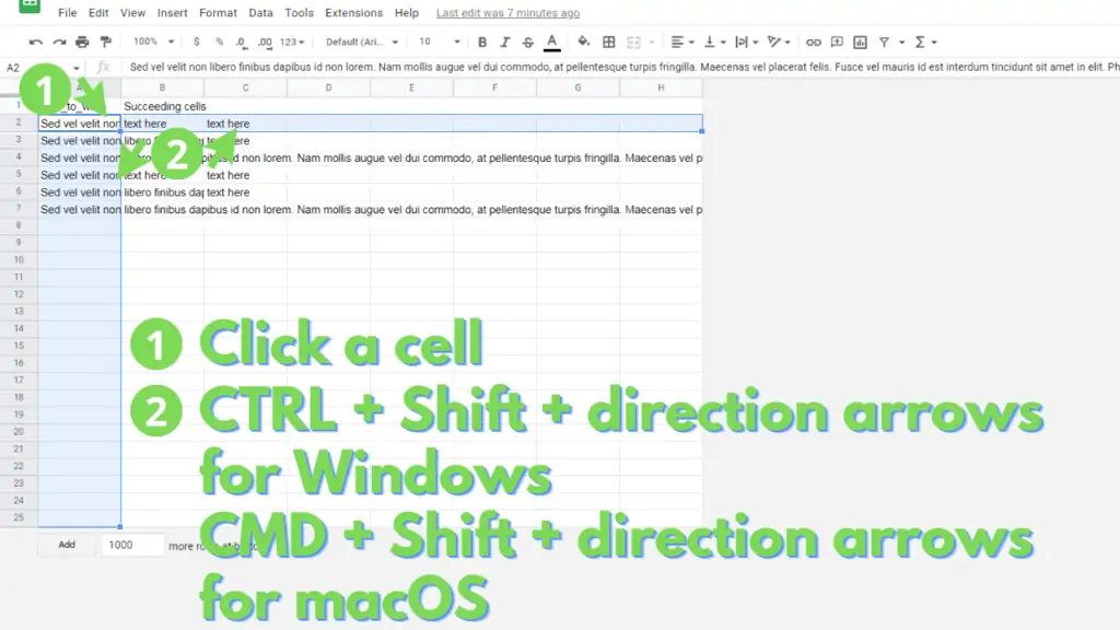
You can select a cell by clicking on it. Alternatively, you can select a range by click-dragging from the first cell to the last cell of your intended range.

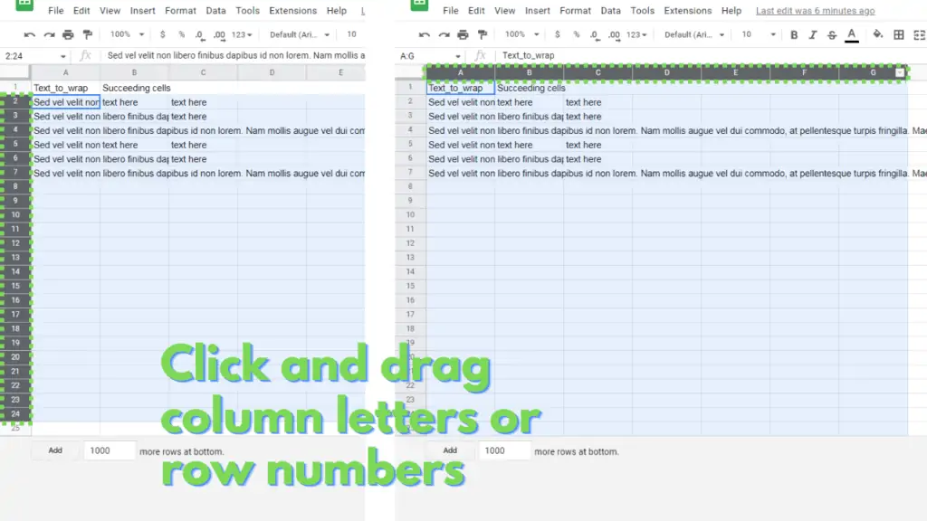
Click or click-drag to select a cell or range

You can also select whole columns or rows by clicking or click-dragging through the column letters or rows numbers.

Click or click-drag column letters or row numbers to select columns or letters

You can select all the cells before or after a certain cell by first selecting a cell, then by holding the Ctrl and Shift keys by pressing the arrow key (up, down, left, or right) that corresponds to which direction from the selected cell you want to select additional cells for.

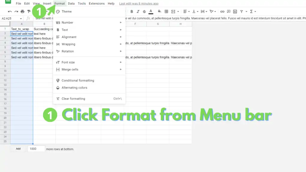
Ctrl + Shift + arrow key to select all cells after a certain cell (PC)

Step 2 – Open the Format Menu

The next step involves opening the Format menu to access the wrapping option. To do this, click on “Format” from the Menu bar.

You can also hold alt then press “o” on your keyboard.

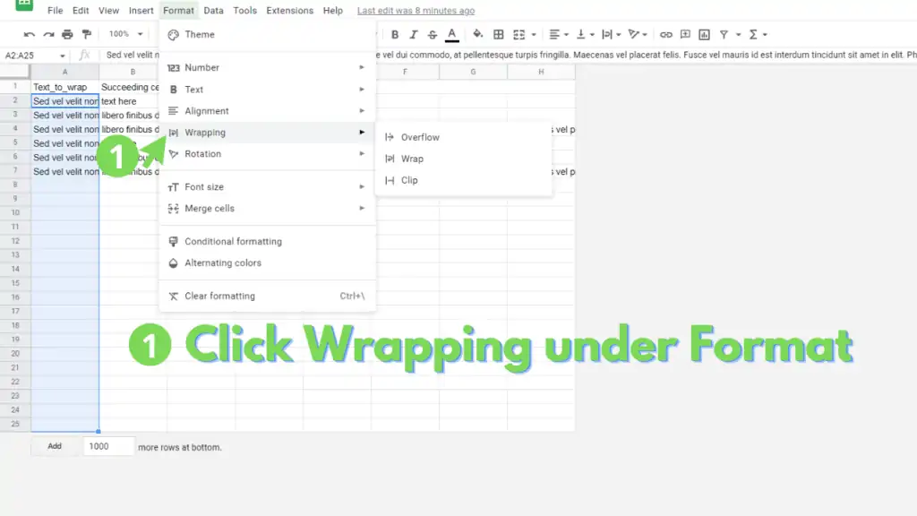
Step 3 – Open the Wrapping Format Option

The next step involves opening the Wrapping format option to access the different wrapping methods.

To do this, hover over or click Wrapping from the Format bar or press “w” on your keyboard.

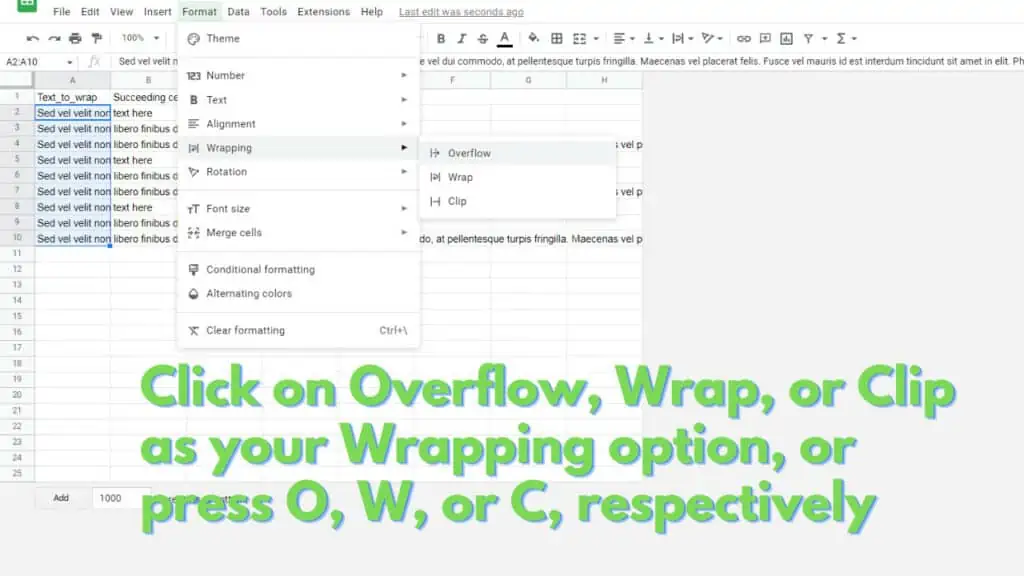
Step 4 – Select a Wrapping Option

The final step in learning how to wrap text in Google Sheets is learning what effects the wrapping options apply to your selection.

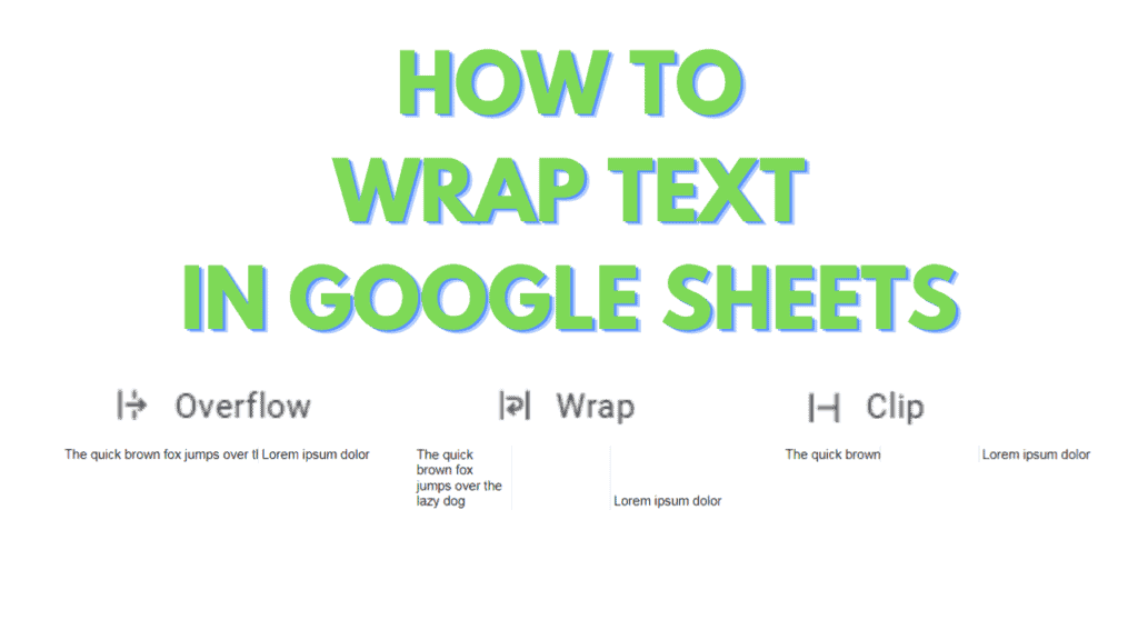
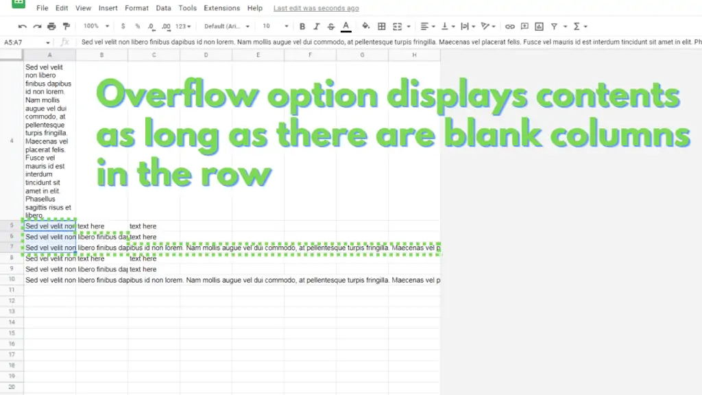
The first wrapping option, “Overflow”, allows the cell to display its contents onto the next cells in its row, but only if the succeeding cells are blank.

Whitespaces and newline characters are considered as values, and thus, cells that contain only them, are not blank. The overflow option is also the default option for all cells in Google Sheets.

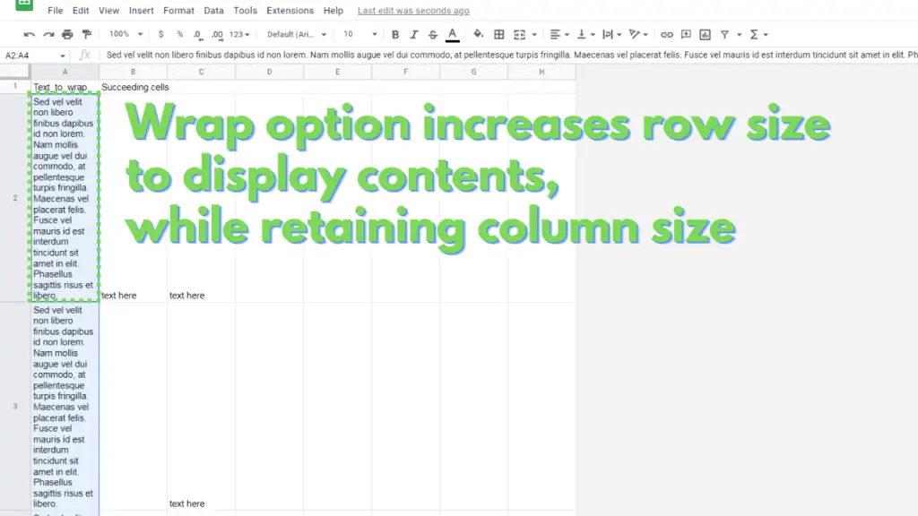
The second wrapping option, “Wrap”, automatically resizes the height of the row that the cell is in if its contents cannot be fully displayed within the original dimensions of the cell.

Furthermore, if the automatic resizing of the row still fails to display the contents of the cell, the cell will be given an extra scroll bar feature, to allow you to view its contents.

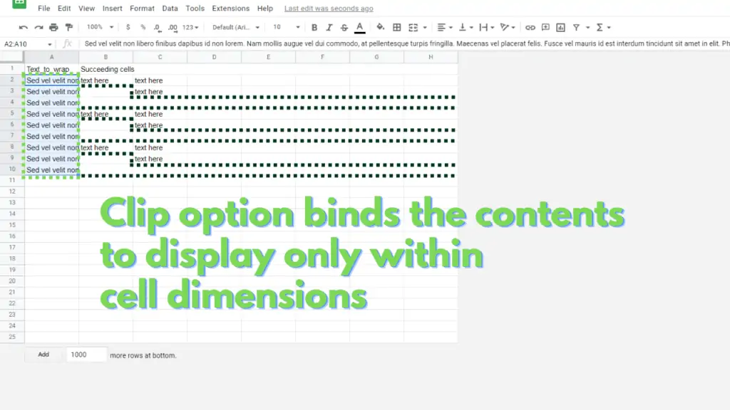
The last wrapping option, “Clip”, restricts values in the cell to only be displayed within the dimensions of the cell, regardless if the succeeding columns in the row are blank.

After learning what effects the wrapping options apply on your selection, you can now select your choice by clicking on any of the options, or by pressing “o”, “w”, or “c” for Overflow, Wrap, or “Clip” respectively, when you have the Wrapping options open from the Format menu.

Text Wrapping in Google Sheets Examples

Overflow wrapping example:

Wrap wrapping example:

Clip wrapping example:

Read about how to auto sort in Google Sheets next.

Frequently Asked Questions on How to Wrap Text in Google Sheets

How do I wrap text in Google Sheets?

First, select the cell or range that you want to apply wrapping options on. Next, open the Wrapping options by clicking Format from the Menu bar. Finally, select your choice of wrapping by either clicking on Overflow, Wrap, or Click, or by pressing “o”, “w”, or “c” respectively.

I’m trying to apply wrap as a wrapping option, but only clip and overflow work. Is this a bug in Google Sheets?

This is not a bug, but an interaction between different options that apply roughly the same effect. The row that you’re trying to wrap may have been manually resized, which overrides the “wrap” option’s ability to resize the row. To remedy this, select all the rows on your worksheet (doing it through the name box is easiest), then resize them, picking “fit to data” as your option. After this, you can wrap your cells again.

I wrapped a column but some cells are expanding even though they shouldn’t, how can I avoid this in Google Sheets?

Check if there is a new line character on the contents of the cell. Google Sheets will treat a new line as its own line even if there aren’t any characters after it, and as such, will take up a display area for your cell. This forces a cell with wrap as its wrapping option to expand its row size.

Conclusion on How to Wrap Text in Google Sheets

Select the cell or range that you want to apply wrapping on. Next, open the Wrapping options by clicking on Format from the Menu Bar, then by clicking on Wrapping. Finally, either click Overflow, Wrap, or Clip, or press Alt + o, Alt + w, or Alt + c, respectively.