How to Use XLOOKUP in Google Sheets -7 Easy Steps

In this tutorial, I will show you how to use XLOOKUP in Google Sheets.

The XLOOKUP function is a new addition to Google Sheets’ suite of lookup functions. It’s best described as a smarter implementation of the HLOOKUP and VLOOKUP in Google Sheets and to an extent the INDEX & MATCH formula implementation.

It eliminates the strict requirement for both the VLOOKUP and HLOOKUP functions to have the search key be in the first row or column of the range, something the INDEX & MATCH formula addresses.

As an improvement to the INDEX & MATCH formula, the XLOOKUP function potentially lessens the burden on both the user and the Google Sheets application. It can return multiple values across a row or column using a single formula.

XLOOKUP in Google Sheets Syntax

The syntax for the XLOOKUP function is:  XLOOKUP(search_key, lookup_range, result_range, missing_value, match_mode, search_mode)

How XLOOKUP in Google Sheets Works Video Tutorial

How to Use the XLOOKUP Function in Google Sheets

To use the XLOOKUP Function in Google Sheets:

1. Identify the [search_key] and [lookup_range] by comparing common values between the source range and the destination range
2. Identify the [source_range]
   1. Return a single value as the [source_range] by providing a single column or row from the source range
   2. Return multiple values from the [source_range] by providing multiple columns or rows as the source range
   3. Reorder the returned values from the [source_range] through the use of an array
3. Create an XLOOKUP formula by substituting [search_key], [lookup_range] and [result_range] with the identified row(s) or column(s)
4. Specify a value to return if no match is found between the [search_key] and the [lookup_range]
5. Specify a number between -1, 0, 1, and 2 that represents the [match_mode] the XLOOKUP function will use for the [search_key] and the [lookup_range]
6. Specify a number between -2, -1, 1, and 2 that represents the [search_mode] the XLOOKUP function will use for the [search_key] and the [lookup_range]
7. Copy the constructed XLOOKUP formula across the rows or columns of the destination range

The XLOOKUP Function Syntax in Google Sheets Explained

The syntax is:

=XLOOKUP(search_key, lookup_range, result_range, missing_value, match_mode, search_mode)

• search_key: The value that XLOOKUP will search for from the lookup_range
• lookup_range: The range that will be searched by the XLOOKUP function
• result_range: The range that will be used by the XLOOKUP function to return a value, depending on the lookup_range where a match has been found for the search_key.
• missing_value: The value returned by the XLOOKUP function when a match cannot be found between the search_key and the lookup_range. Can be a text, a number, or a boolean. Defaults to an error when not specified.
• match_mode: The type of match to be used when searching for the search_key from the lookup_range. Can be -1, 0, 1, or 2. Defaults to 0 when not specified. 0 will return exact matches only. -1 will look for the smallest item if no exact match is found. 1 looks for the exact match or the next greater value. 2 can be selected for wildcard match.
• search_mode: The searching method used when searching for the search_key from the lookup_range. Can be 1, -1, 2, or -2. Defaults to 1 when not specified. 1 stand for a search from the first to the last entry. -1 stands for a last to first entry search. 2 is for binary search working with an ordered list. -2 is for binary search as well but for list arranged in descending order

XLOOKUP in Google Sheets Step-By-Step Examples

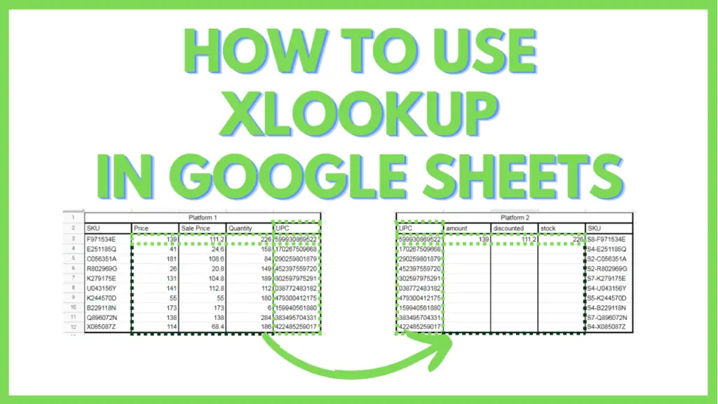
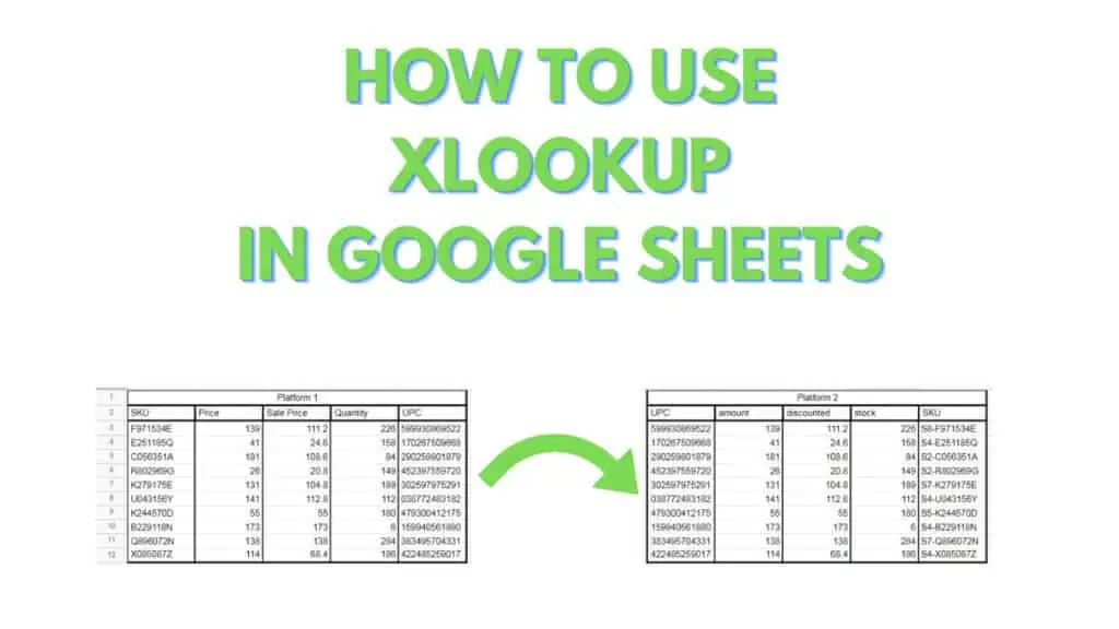
For this tutorial, I will provide a sample file that will have 2 worksheets.

The first worksheet simulates a typical export of data from an eCommerce platform, while the second will contain an incomplete table that we will build according to the import requirements of a different eCommerce platform.

You can make a copy of the file by accessing it through this link, then by clicking on “File” from the Menu Bar, then by clicking on “Make a copy”.

A dialog box should appear. Within it, you can provide a filename for the Copy then click “Make a Copy”.

Step 1 – Identify the [search_key] and [lookup_range] by comparing common values between the source range and the destination range

By observing the data from the sample that I provided, you can observe that the UPC column for both sheets has similar values: 12-digit combinations with leading zeroes.

There are several ways to check the veracity of this observation, but one of the easiest methods I personally use, is this formula:

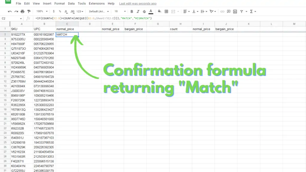
=IF(COUNTA(B2:B)=COUNTA(UNIQUE({B2:B;Sheet1!E2:E})),”MATCH”,”MISMATCH”)

The formula above counts the unique values of the current sheet’s B2:B range, then compares it with the count of unique values of both the current sheet’s B2:B range and Sheet1’s E2:E range. If the values are equal, then it returns a “MATCH” text, otherwise, it will return “Mismatch”.

Copy and paste the formula to any cell on Sheet2 of your copy of the sample file I provided.

It should return a value of “MATCH”, confirming our earlier observation, and subsequently identifying the UPC column for both sheets as the [search_key] and [lookup_range] parts for our XLOOKUP formula.

Using this information, our formula should start to like this:

=XLOOKUP(B2,Sheet1$E$2:E,[result_range],[missing_value],[match_mode],[search_mode]

Step 2 – Identify the [source_range]

The next step involves further evaluation of what data we need returned by the XLOOKUP function.

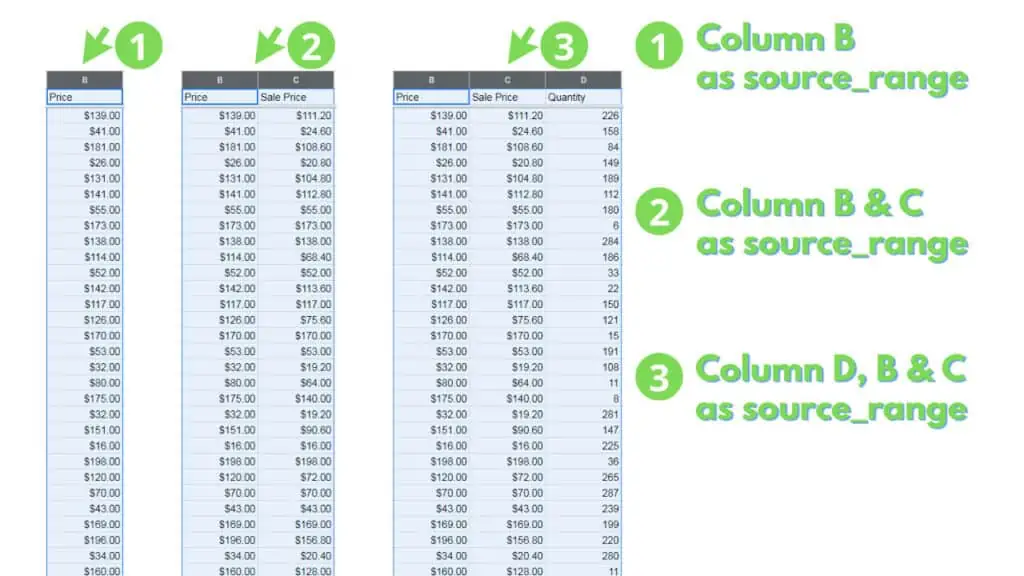
On Sheet2, we can observe on column C that we’re looking for a monetary value, and by comparing what values can be extracted from Sheet1, we can narrow it down to only 2 columns that present monetary values: column B with “Price”, and column C as “Sale Price”. Logically, the result range would be column B from Sheet1 or “Sheet1!$B$2:$B”.

The next group, found on columns E and F of Sheet2, are logically columns B and C from Sheet1 or “Sheet1!$B$2:$C”.

The last group, found on columns H to J of Sheet 2, are columns D, B and C from Sheet1, respectively. However, unlike the previous 2 cases, we cannot use “Sheet1!B2:D” as the result range, because it would return columns B, C, and D, in that order.

Alternatively, we can construct 2 XLOOKUP formulas, one that uses Sheet1 column D as the result range, and another that uses Sheet1 columns B and C as the result range.

This, however, can be simplified by the use of a single XLOOKUP function that returns 3 non-consecutive columns or rows, through the use of an array. The following syntax organizes columns D, B, and C from Sheet1 in an array:

{Sheet1!$D$2:$D,Sheet1!$B$2:$C}

Step 3 – Create an XLOOKUP formula by substituting [search_key], [lookup_range] and [result_range] with the identified row(s) or column(s)

Guided by what you’ve observed from the previous steps, you can now create a simple XLOOKUP formula.

To return column B from Sheet1 as a single value, the syntax would look like the following:

=XLOOKUP(B2,Sheet1$E$2$:E,Sheet1$B$2:$B,[missing_value],[match_mode],[search_mode])

To return columns B and C from Sheet1 as 2 consecutive values in a single row, the syntax would look like the following:

=XLOOKUP(B2,Sheet1$E$2:$E,Sheet1$B$2:$C,[missing_value],[match_mode],[search_mode])

To return columns D, B and C from Sheet1, in that specific order, as consecutive values in a single row, the syntax would look like the following:

=XLOOKUP(B2,Sheet1!$E$2:$E,{Sheet1!$D$2:$D,Sheet1!$B$2:$C},[missing_value],[match_mode],[search_mode])

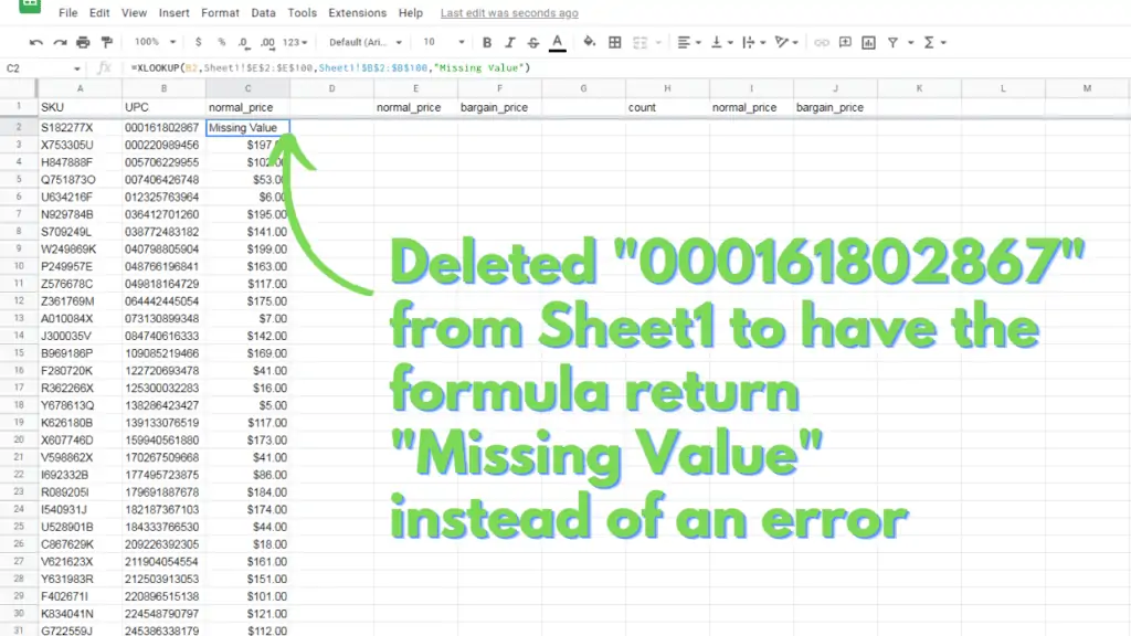
Step 4 – Specify a value to return if no match is found between the [search_key] and the [lookup_range]

Next, we move on to the optional parts of the XLOOKUP formula, the first of which is the [missing_value].

The missing value part of the XLOOKUP formula allows you to specify a returned value if your [search_key] does not match any value from the [lookup_range].

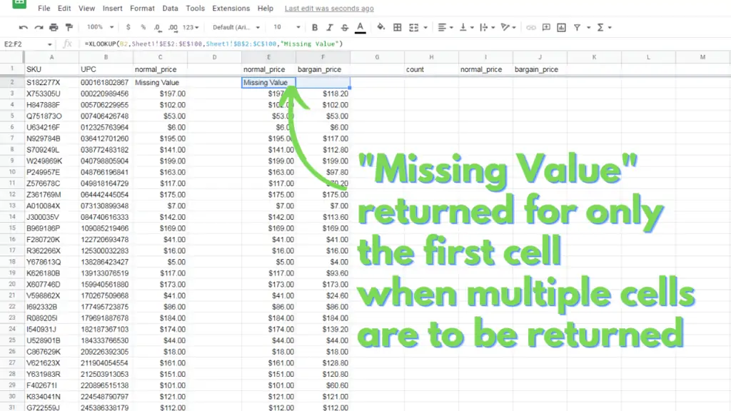
When using an XLOOKUP formula that is supposed to return multiple rows or columns as values, the specified [missing_value] would only appear on the left-most or top-most cell.

If this option is left blank, an error is returned for a [missing_value].

Step 5 – Specify a number between -1, 0, 1, and 2 that represents the [match_mode] the XLOOKUP function will use for the [search_key] and the [lookup_range]

Next is another optional part of the XLOOKUP formula, the [match_mode].

Enter the value -1 if you are looking for an exact match of your [search_key], or the next value that is bigger than your [search_key].

Enter the value 0 if you are looking for an exact match only.

Enter 1 if you are looking for an exact match of your [search_key], or the next value that is lower than your [search_key]
Or, enter 2 if you are looking for an exact match of your [search_key] but would like to return wildcard matches if no exact match is found.

If this optional part is left blank, the formula defaults to searching for an exact match only.

Step 6 – Specify a number between -1, 1, -2, and 2 that represents the [search_mode] the XLOOKUP function will use for the [search_key] and the [lookup_range]

The final optional part of the XLOOKUP formula is the [search_mode].

Enter the value -1 to have the formula search through the [lookup_range] from the last value to the first (right to left for rows, then bottom to top for columns).

Enter the value 1 to have the formula search through the [lookup_range] from the first value to the last (left to right for rows, then top to bottom for columns).

Enter the value -2 to have the formula perform a binary search through the [lookup_range] assuming that the [lookup_range] is first sorted in descending order.

Enter the value 2 to have the formula perform a binary search through the [lookup_range] assuming that the [lookup_range] is first sorted in ascending order.

If this optional part is left blank, the formula defaults to searching through the [lookup_range] from the first value to the last.

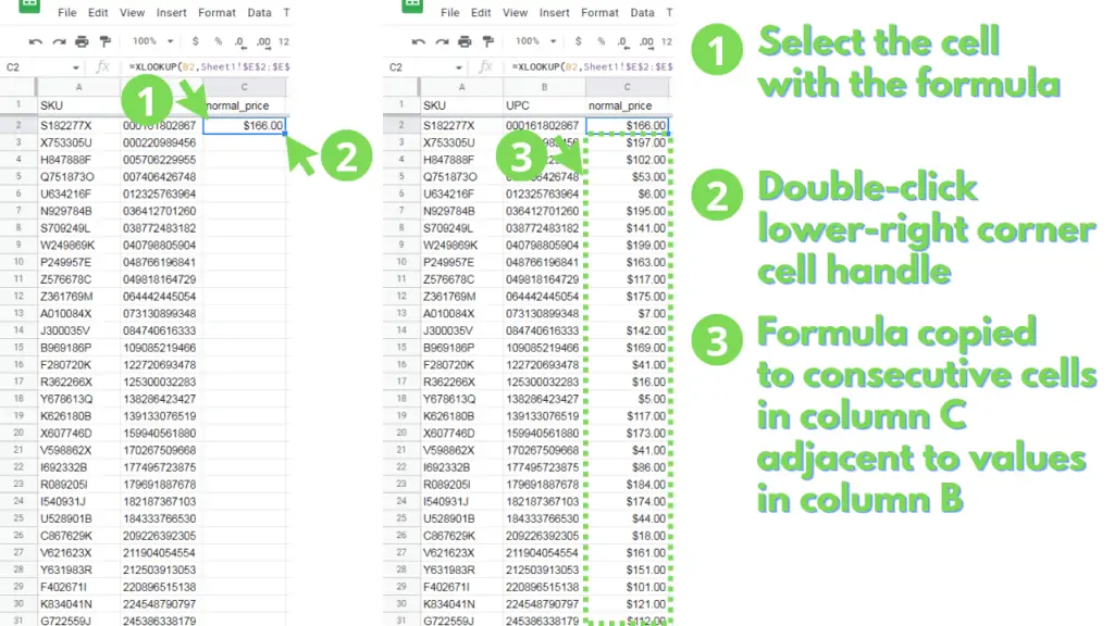
Step 7 – Copy the constructed XLOOKUP formula across the rows or columns of the destination range

Now that you’ve constructed your own XLOOKUP formulas, you can copy them onto the rest of their respective rows along a column.

The first method to do this is by simply selecting the cell with the formula, then by double-clicking the square at the bottom-right corner of the cell.

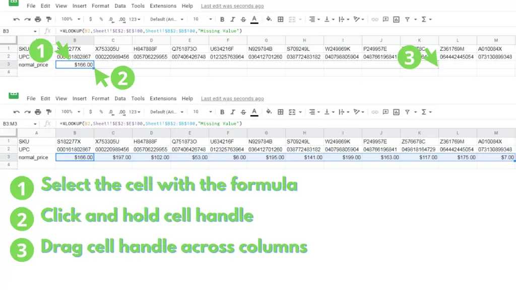
If, however, you’re trying to copy the formula across columns along a cell, common when using an HLOOKUP or an XLOOKUP on a horizontal profile, you will need to select the cell then drag its lower-right corner along the columns of the row.

Copying (CTRL + C) and pasting (CTRL + V) will work in copying the formula across columns of a row or along rows of a column.

XLOOKUP in Google Sheets Examples

Use an XLOOKUP to return the value in Sheet1 range B2:2, using a search_key from Sheet2 B2, through the lookup_range in Sheet1 B1:1.
=XLOOKUP(Sheet2!B2,Sheet1!B1:1,Sheet1!B2:2)

Use an XLOOKUP to return values in Sheet1 range D2:F, using a search_key from current sheet B2, through the lookup_range in Sheet1 G2:G, returning the text “No Match” for missing values, using wildcard as match_mode, and bottom to top as search_mode.
=XLOOKUP($B2,Sheet1!$G$2:$G,Sheet1!$D$2:$F,”No Match”,2,-1)

Use an XLOOKUP to return values in sheet “raw import” range A2:G, using a search_key from current sheet C2, through the lookup_range in Sheet1 C2:C, returning the text “No match found” for missing values, using default exact match as match_mode, and default top to bottom as search_mode.
=XLOOKUP($C2,’raw import’!$A$2:$G,Sheet1!C2:C,”No match found”)

Frequently Asked Questions on how to use XLOOKUP in Google Sheets

Conclusion How to use XLOOKUP in Google Sheets

Identify the [search_key] and [lookup_range] by comparing common values between the source range and the destination range.

The search key is a single cell address (A2, B2, C2, etc.), while the lookup range is a range address for a single column or row ($A$2:$A, $B$2:$2, etc.)

Identify the [source_range] that values will be taken from if a match is found between the [search_key] and the [lookup_range]. It can be a single value from a row ($D$2:$D) or column ($B$2:$2).

It can be multiple values across rows ($D$2:$E) or along columns ($D$2:$3). And, it can also be an array that reorders the returned values across rows ({$F$2:$F,$D$2:$E}) or along columns ({$B$4:$4;$B$2:$3}).

Create your XLOOKUP formula by substituting [search_key], [lookup_range] and [result_range] with the identified row(s) or column(s) for the formula:
(“=XLOOKUP([search_key],[lookup_range],[source_range])”)

Optionally specify a value and substitute to [missing_value] if no match is found between the [search_key] and the [lookup_range] for the formula:
(“=XLOOKUP([search_key],[lookup_range],[source_range],[missing_value])”)

Optionally specify a number between -1, 0, 1, and 2 and substitute to [match_mode] where -1 searches for an exact match or the next lower value, 1 searches for an exact match or the next higher value, 0 searches only for an exact match, and 2 searches for wildcard match if no exact match is found:

(“=XLOOKUP([search_key],[lookup_range],[source_range],[missing_value],[match_mode])”)

Optionally specify a number between -1, 1, -2, and 2 and substitute to [search_mode] where -1 searches through the [lookup_range] from the last value to the first, 1 searches through the [lookup_range] from the first value to the last, -2 performs a binary search assuming that the [lookup_range] is in descending order, and 2 performs a binary search assuming that the [lookup_range] is in ascending order.

(“=XLOOKUP([search_key],[lookup_range],[source_range],[missing_value],[match_mode],[search_mode])”)

Finally, copy the XLOOKUP formula along a column by double-clicking the lower right corner of the cell, or by dragging the cell across a row or along a column.