Can you imagine the nightmare of scrolling through thousands of rows or clicking ‘Next’ endlessly when you use the Find function in Google Sheets?
I’ve been using spreadsheets for more than 20 years now and I can say VLOOKUP is one of the more advanced functions anyone should know how to use.
In this tutorial, I am going to show you how to use VLOOKUP in Google Sheets and how you can use it to find data in different scenarios.
How to Use VLOOKUP in Google Sheets
- Set up a search key
- Prepare your reference dataset with the search column at the leftmost part of the range
- Identify which column will be returned as the index
- Use the formula: “=VLOOKUP(search_key, range, index, [is_sorted])”
How to Use VLOOKUP in Google Sheets Video Tutorial
Basics of VLOOKUP in Google Sheets
The syntax of VLOOKUP in Google Sheets is:
VLOOKUP(search_key, range, index, [is_sorted])
- search_key – the value to be looked for in the range.
- range – the reference dataset, its first column should contain the index
- index – the column index in the range to be returned, the first column of the range is ‘1’
- [is_sorted] – optional parameter to indicate if the search column is sorted. This is TRUE by default. For most cases, it’s useful to set this as FALSE.
It is also important to note that if there are multiple returns to a VLOOKUP in Google Sheets, it will only return the first match.
A Common Error Using The VLOOKUP in Google Sheets is “vlookup evaluates to an out of bounds range”
When the VLOOKUP function returns an error that says “vlookup evaluates to an out of bounds range” it means that there is an error in the formula used.
The two most common causes for this error to appear are a #REF error caused by a range that is too short or when the index is greater than the selected range.
I dedicated a whole article to vlookup evaluates to an out of bounds range in Google Sheets.
3 Ways On How to Use VLOOKUP in Google Sheets – Step-By-Step
There are a lot of ways how to use VLOOKUP in Google Sheets.
In this tutorial, I’m going to talk about three of the most useful ones that I often use.
I’ll use a personnel file dataset to demonstrate these different ways in Google Sheets.
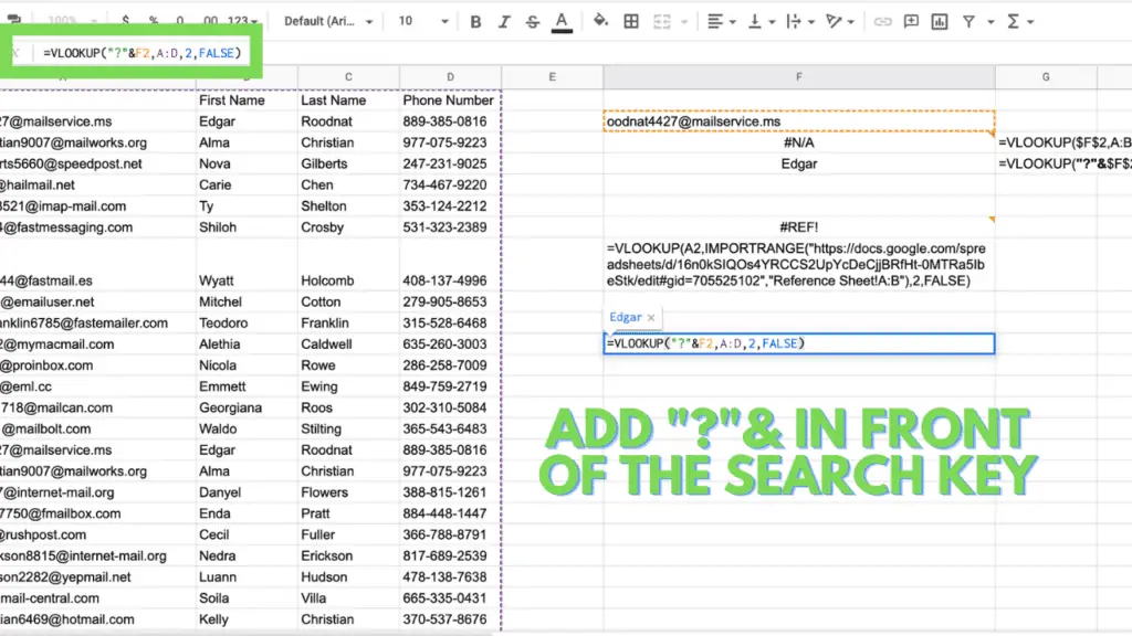
VLOOKUP Using Wildcard Characters in Google Sheets
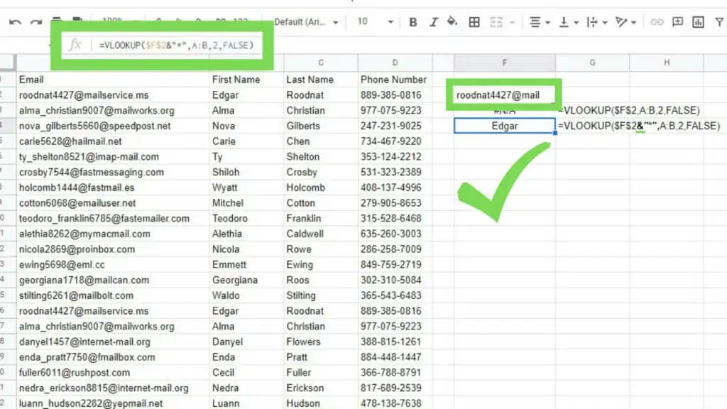
The most crucial part that defines your search using VLOOKUP in Google Sheets is the search_key. And sometimes, it’s not as defined as you may want it to be. Or, depending on the situation, it is great if it is a little vague.
In these scenarios, we can use “Wildcard Characters” such as an asterisk (*) and a question mark (?) to indicate the wildcard property of the search_key.
The asterisk (*) wildcard character lets VLOOKUP search for a sequence of characters instead of a full string or word.
For example, the search term “Cat*” can accept “Cat”, “Cate”, “Cat123”, “Catnip”, and any other term with “Cat” at the start of it.
The question mark (?) wildcard character lets VLOOKUP search for the search_key with an unknown character before it.
For example, the search term “?eat” can accept “Heat”, “Peat”, “1eat”, “@eat”, and any other term with “eat” at the end of it.
I find it important to mention that even though the wildcard characters are useful in getting more results, especially for cases where you’re not sure of the exact value of the search_key, it’s not the most accurate method.
Both the asterisk (*) and question mark (?) in search_keys will let VLOOKUP return the first value that will match it and not necessarily the right one 100% of the time.
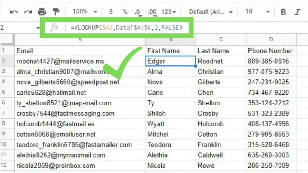
VLOOKUP Using a Range from a Different Sheet
One of the most useful applications of VLOOKUP in Google Sheets is that you can use it to search for data from one sheet and present it in another spreadsheet.
This way, you’ll have a cleaner sheet where you can present only the data that you want to display.
I made a smaller dataset below from the Personnel file dataset sample using email addresses as the search_key.
This way, I can “clean” the data and only display the email address for each employee, the first name, last name, and phone number.
How to Use VLOOKUP in Google Sheets Using a Range from a Different Workbook
VLOOKUP in Google Sheets can also be used to search in ranges found in a different workbook by using the IMPORTRANGE Function.
Just replace the range parameter with the range imported by using the IMPORTRANGE Function.
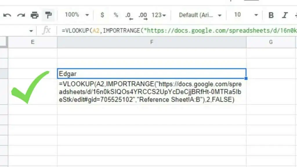
When using the IMPORTRANGE function for the first time, a #REF! will be returned and the notice message below will show up.
This is because you need to grant the IMPORTRANGE function access to connect sheets for the first time.
Just hit ‘Allow access’ to continue.

This is how you use VLOOKUP in Google Sheets with ranges from different sheets in the same or even from a different workbook.
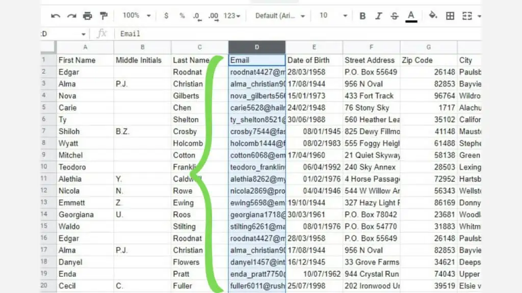
VLOOKUP Using a Misplaced Search Column in Google Sheets
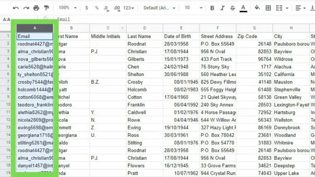
When using VLOOKUP, your range must have the search_key column as its first parameter.
Meaning, if you’re running the VLOOKUP Function to extract first names by using email addresses, the latter should be the 1st column of your range.
That said, if in case you are in a situation where you don’t have the search_key column at its proper position, and you can’t make any changes to the source dataset by moving the columns around, you may find yourself in a tough spot.
In that case, you can create a new sheet and reference the source dataset. This way you can then use the new sheet as your range.
Alternatively, you can use my method which is simpler and does not require adding more sheets.
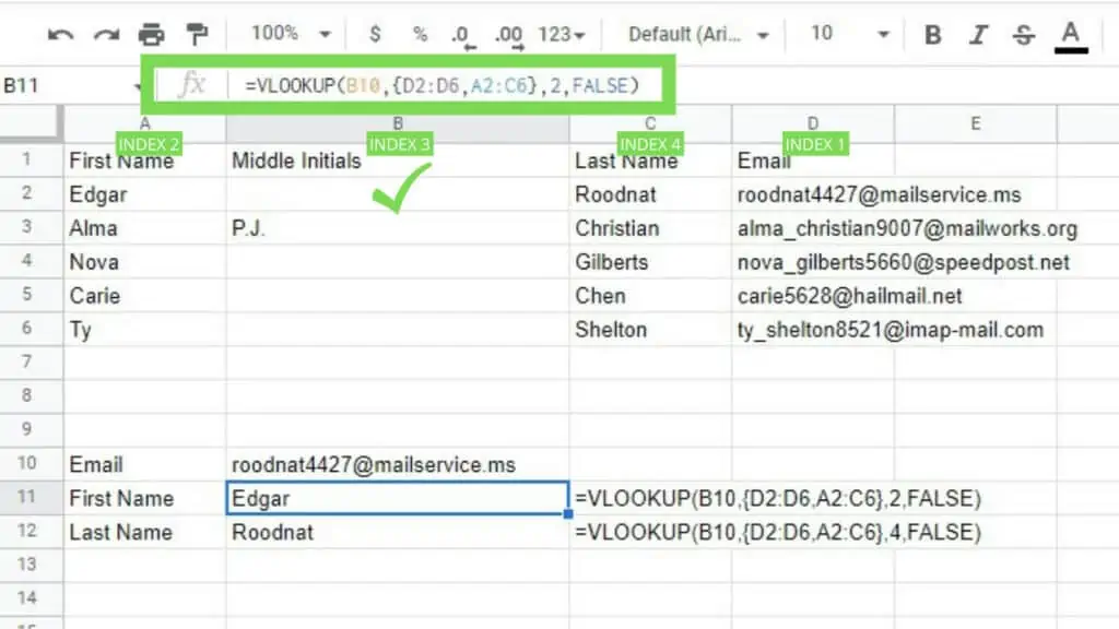
To do this, you just need to modify the range parameter to be {search_range,lookup_range}
For the example below, I have a small dataset with the range A1:D6.
That said, since my search_key is each row’s email, I won’t be able to use it as it is since it’s not on the first column.
So applying my method to this situation, I can just use the formula below:
=VLOOKUP(B10,{D2:D6,A2:C6},2,FALSE)
D2:D6 being my search_range and A2:C6 being my lookup_range.
For the index parameter, you’ll have to consider the search_range being the 1st column and will have the index 1, while the look_up range starts at index 2.
These are the most useful use cases of VLOOKUP in Google Sheets.
How to Vlookup from a Different Sheet
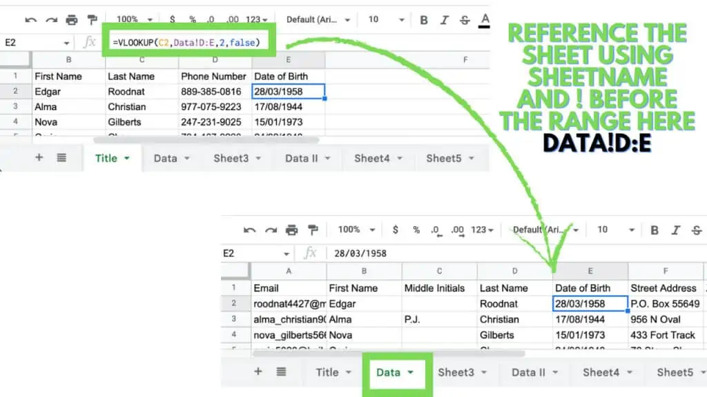
To use Vlookup from a different sheet set the name of the sheet in front of the range and put an exclamation mark (!) right after the sheet name.
The syntax is:
‘Sheet Name’!Range
Example: VLOOKUP(C2,Data!D:E,2,false)
The VLookup will lookup C2 which is the name “Roodnat” in Sheet Data within the range D:E. 2 is the Index, so column 2 in the range carries the Date of Birth.
The correct date of birth “28/03/1982” is thus displayed in Sheet Title.
If the sheet name has any special characters or spaces in the name, make sure to encapsulate it within single quotation marks (‘ ‘) like in this example: ‘Data Set!D:E’.
Vlookup Using the INDEX MATCH Formula in Google Sheets for Left Vlookup
When using the Vlookup function you may have realized that it can only look up values in the first column that is within the lookup range.
This is a limitation that can be overcome by using the INDEX MATCH formula in Google Sheets.
The syntax for the INDEX MATCH formula is:
=INDEX(range1,MATCH(search_key,range2),0))
An example of the Index and Match function is given below.
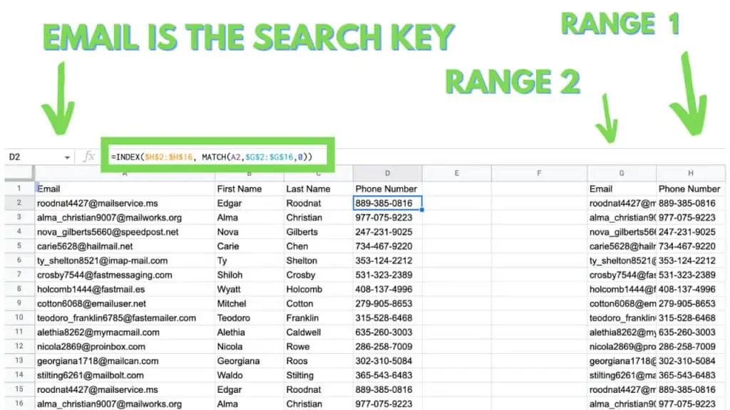
In the example, I am looking up the phone number using the email address of people.
The email address is the “Search Key”.
“Range1” is where the phone numbers are.
“Range2” defines where the email addresses and thus the “lookup value” can be found that we want to match.
The last value “0” is the search method.
0 finds an exact value when a range is unsorted.
1 would find the largest value that is less or equal. For this, we would need a sorted list in ascending order.
Most lists are not in ascending order thus usually 0 is used.
There is also the value -1 which stands for the smallest value that is equal to or greater than the “Search Key”.
-1 can be used when the list is ordered in descending order.
One of the biggest advantages of using the Index and Match function over the index function is that it doesn’t matter if columns are deleted or rearranged.
Since this formula does not rely on a specific order, it will be automatically updated. This is why it can be regarded as a better alternative to the Vlookup function in Google Sheets as it cannot look to its left.
Frequently Asked Questions about How to Use VLOOKUP in Google Sheets
How do I use the IF Function with VLOOKUP in Google Sheets?
You can use IF and VLOOKUP in Google Sheets by replacing the range parameter of VLOOKUP with the IF Function. You can also use a combination of IFERROR and VLOOKUP to display a custom message explaining the error like “No record”.
Can I search for case-sensitive terms with VLOOKUP in Google Sheets?
You cannot use VLOOKUP to search for case-sensitive terms in Google Sheets. Instead use this formula: ArrayFormula(INDEX(return_range, MATCH (TRUE,EXACT(lookup_range, search_key),0))) where return_range is the column address for the index parameter and lookup_range is the search_range of VLOOKUP.
Conclusion on How to Use VLOOKUP in Google Sheets
To Use VLOOKUP in Google Sheets, set up a search key and prepare your reference dataset with the search column at the leftmost part of the range. Then, identify which column will be returned as the index. Lastly, use the formula: “=VLOOKUP(search_key, range, index, [is_sorted])”.

