In this tutorial, I will teach you how to use TRANSPOSE in Google Sheets.
How to use TRANSPOSE in Google Sheets
To use TRANSPOSE in Google Sheets:
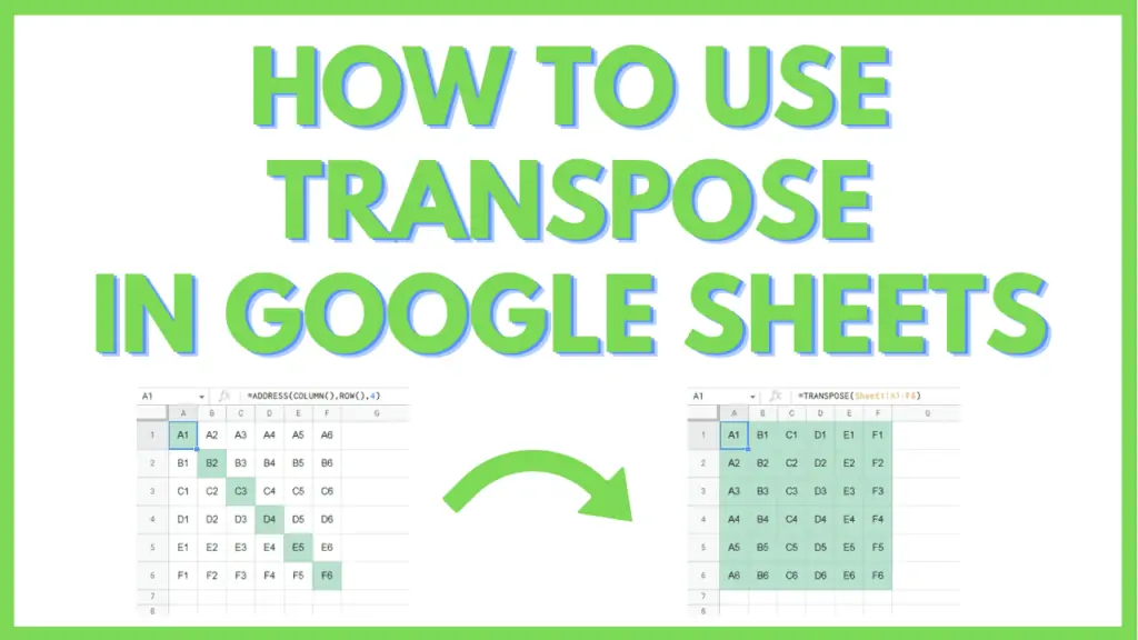
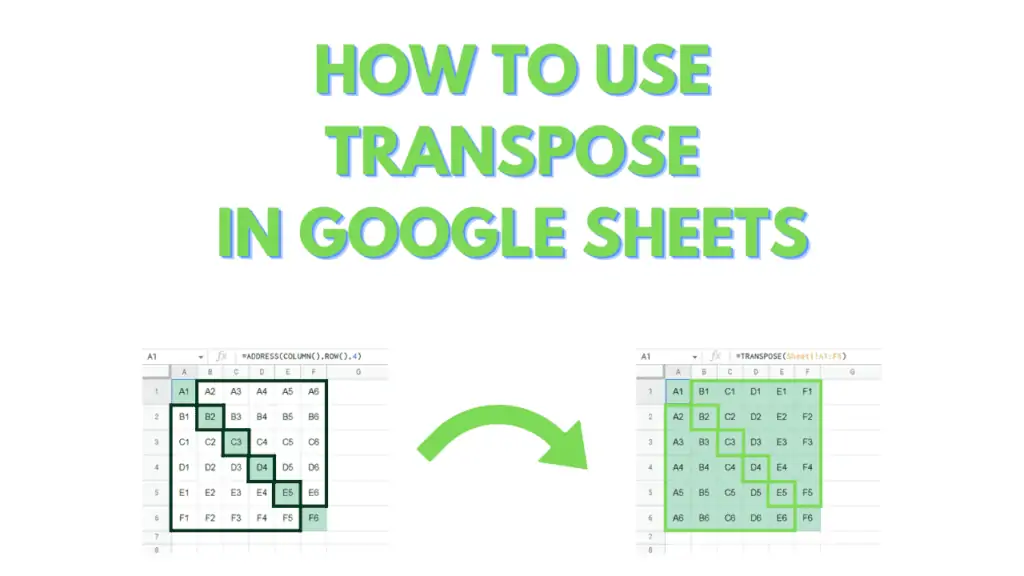
- Transpose a range to switch its rows into columns and vice versa by using =TRANSPOSE([Range])
- Transpose an array to switch its rows into columns and vice versa eg. =TRANSPOSE({‘Unorganized Data’!A1:2;’Unorganized Data’!A4:4})
- Transpose an array and force a row or a column into the desired position eg. =TRANSPOSE({‘Unorganized Data’!A2:2;’Unorganized Data’!A5:6})
TRANSPOSE in Google Sheets – The Basics
The TRANSPOSE function is an array function that reorganizes a range or an array by switching its columns into rows, or vice-versa.
This is especially useful in repurposing data to have your choice of header rows or header columns, without manually moving the selected range to be positioned in the first row or column.
This is because manually moving around rows or columns will not affect formulas that are referencing the original rows or columns. Moving column C to column A, will not update a formula that already references column A, even if it uses an absolute reference.
Another common scenario where the TRANSPOSE function in Google Sheets shines is in adding formulas that you want to apply to whole rows.
As you may have noticed, it’s far easier and more convenient to apply a single formula down a column than across a row.
This is because you can simply double-click the lower-right corner of a cell to apply the formula down a whole column, instead of copying or dragging a formula across a row.
It is more prudent to transpose a table so that you are applying the formula down a column than it is across a row.
Through the use of the TRANSPOSE function, you will find it easier to simply flip or reorganize your data for post-processing, instead of modifying Pivot Chart setups, Time Calculation formulas, Substring Manipulation, etc. in Google Sheets.
TRANSPOSE in Google Sheets Example Step-By-Step
For this tutorial, I will provide a sample file that has 4 sheets.
The first sheet, titled “Unorganized Data”, will contain the raw data that we will manipulate with the TRANSPOSE function.
The 2nd to 4th sheets will serve as blank sheets that we will populate with data from the “Unorganized data” sheet, with various applications of the TRANSPOSE function.
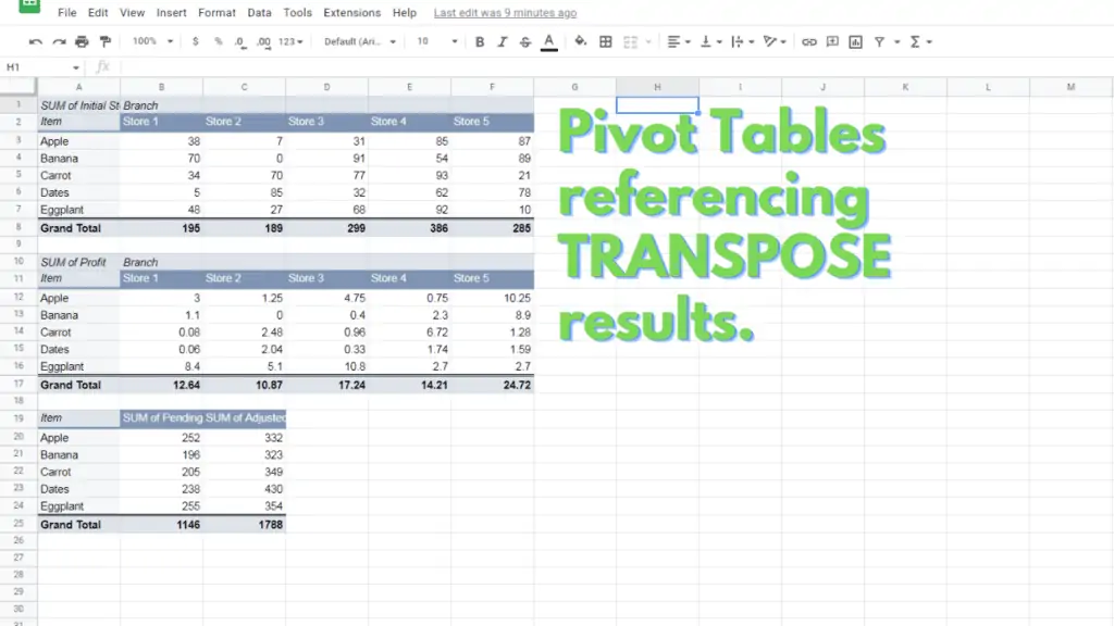
The 5th sheet is a collection of Pivot Tables that refer to ranges in the 2nd to the 4th sheets.
Once we have learned and applied the various methods in using the TRANSPOSE function, the Pivot Tables should work and look like the following:
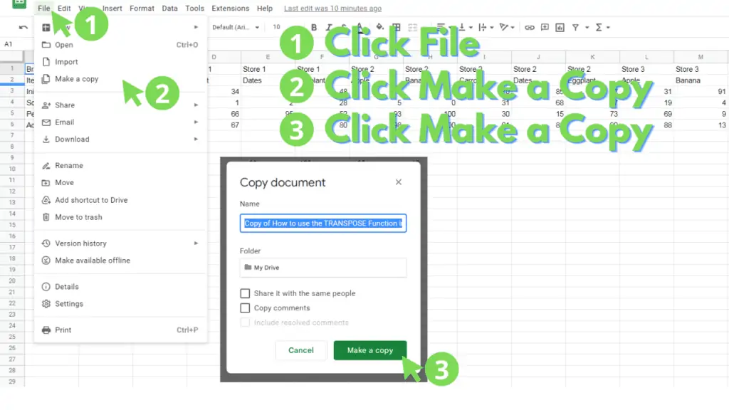
You can make a copy of the file by accessing it through this link, then by clicking on “File” from the Menu Bar, then by clicking on “Make a copy”.
A dialog box should appear. Within it, you can provide a filename for the Copy then click “Make a Copy”.
Method 1 – Transpose a range to switch its rows into columns and vice versa in Google Sheets
This method will teach you how to use the TRANSPOSE function to reorganize data, switching its rows into columns.
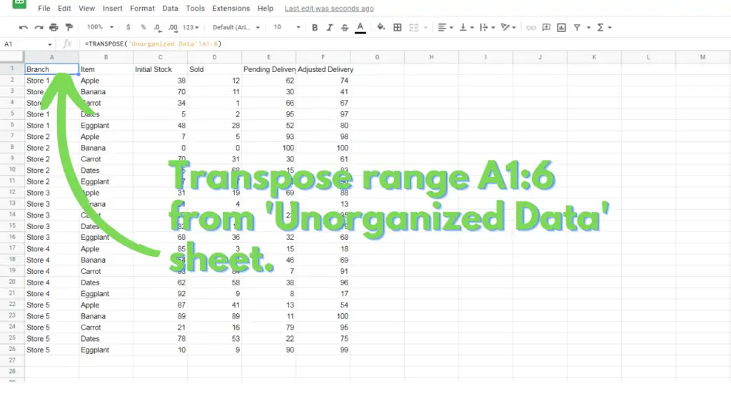
For this, you need to refer to the sheet “Unorganized Data”. You will be using the TRANSPOSE function to reorganize the data, so that the values in rows 1 to 6 will be listed as values in columns A to F in Sheet2.
To do this, substitute the range “’Unorganized Data’!A1:6” to [Range] for the formula and paste it on cell A1 of Sheet2:
=TRANSPOSE([Range])
The formula and result should look like this:
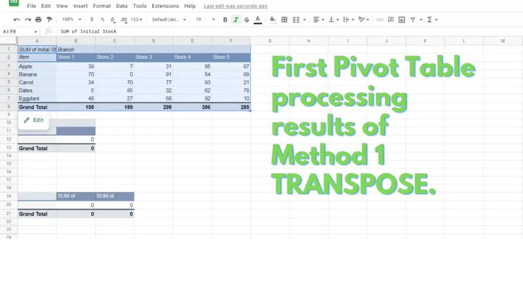
This table will then be referenced by the first Pivot Table in the “Pivot Tables” sheet, which should now look like this:
Method 2 – Transpose an array to switch its rows into columns and vice versa in Google Sheets
This method uses the TRANSPOSE function to reorganize an array of data, switching its rows into columns.
The application of this method will allow you to create a formula that you will apply to a new column. This will be easier than applying the formula across a row.
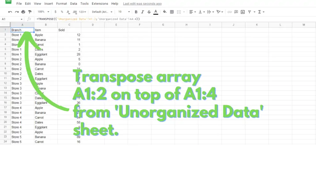
For this, you need to refer to the sheet “Unorganized Data”. You will be using the TRANSPOSE function to reorganize the data, so that the values in rows 1, 2, and 4 will be listed as values in columns A to C in Sheet3.
To do this, substitute the array {‘Unorganized Data’!A1:2;’Unorganized Data’!A4:4} to [Range] for the formula and paste it on cell A1 of Sheet3:
=TRANSPOSE([Range])
The formula and result should look like this:
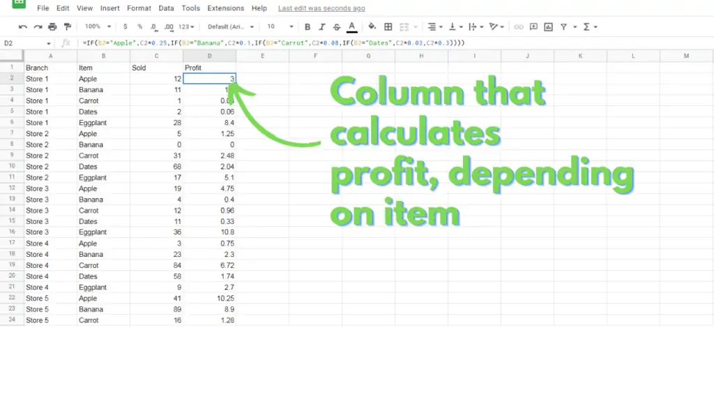
Next, enter the text “Profit” to cell D1 in Sheet3, this will serve as the column header.
Add the following formula to cell D2 in Sheet3, then apply it to the rest of the column:
=IF(B2=”Apple”,C2*0.25,IF(B2=”Banana”,C2*0.1,IF(B2=”Carrot”,C2*0.08,IF(B2=”Dates”,C2*0.03,C2*0.3))))
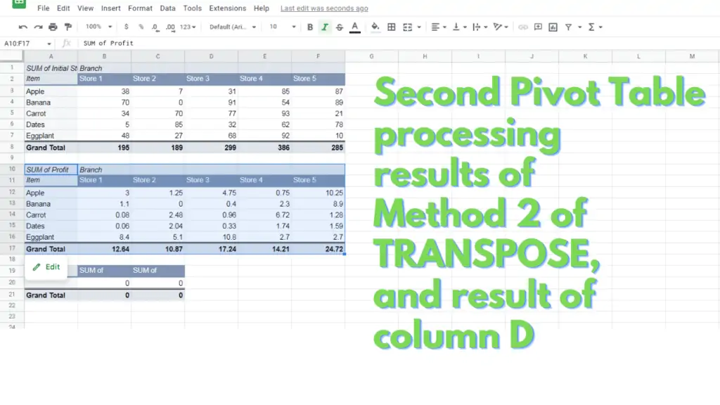
The final result for the table in Sheet3 should look like this:
This table will then be referenced by the second Pivot Table in the “Pivot Tables” sheet, which should now look like this:
Method 3 – Transpose an array and force a row or a column into the desired position in Google Sheets
This method will use the TRANSPOSE function to reorganize an array, forcing the values of a specific row into values under a specific column of a table.
The application of this method will allow you to specify a header row or column for your table.
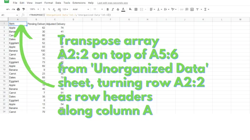
For this, you need to refer to the sheet “Unorganized Data”. You will be using the TRANSPOSE function to reorganize the data, so that the values in rows 2, 5, and 6 will be listed as values in columns A to C in Sheet4.
This essentially places the values in row 2 to be the row headers in Column A.
To do this, substitute the array {‘Unorganized Data’!A2:2;’Unorganized Data’!A5:6} to [Range] for the formula and paste it on cell A1 of Sheet4:
=TRANSPOSE([Range])
The formula and result should look like this:
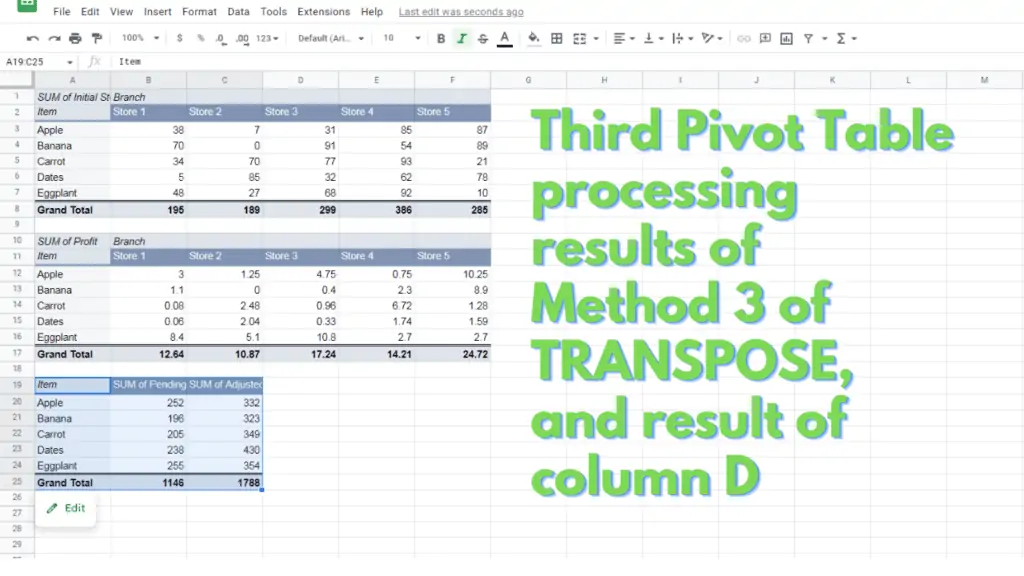
This table will then be referenced by the third Pivot Table in the “Pivot Tables” sheet, which should now look like this:
You now know how to use TRANSPOSE in Google Sheets!
Frequently Asked Questions on How to use TRANSPOSE in Google Sheets
I get an error that says I’m missing values for one or more rows when transposing an array, how do I fix this in Google Sheets?
This error actually stems from how the array itself is constructed. An array works best if the columns within it have an equal number of entries. Array {A1:C1;A2:C2} is generally better than {A1:C1;A2:B2}. Adjust the dimensions of the arrays so they are uniform, before using them in a TRANSPOSE function.
Will the transposed tables expand the dimensions of the worksheet in Google Sheets?
If you transpose a row or a column that would have entries beyond the default dimensions of the sheet (26 columns, 1000 rows), the sheet’s dimensions will automatically adjust to accommodate more entries.
Conclusion on How to use TRANSPOSE in Google Sheets
There are several common applications of the TRANSPOSE function in Google Sheets.
The first application is to use the TRANSPOSE function to switch a range’s rows into columns and vice versa. To transpose the range A1:J2, substitute the address of the range to [Range] of this formula: “=TRANSPOSE([Range])”.
The next application is to use the TRANSPOSE function to make it easier to apply a formula under a new column, instead of applying the formula across a row. Instead of applying a formula that references the range A1:J2 across the row A3:J3, first transpose A1:J2 and then apply a formula that references the resulting range, A1:B10, in column C.
The next application is to use the TRANSPOSE function to use the values of the range A2:J2 as the row headers for the values in range A3:J6. To do this, create an array with A2:J2 as the first row, then the range A3:J6 as the succeeding rows (“{A2:J3;A3:J6}”). Then, substitute the array to [Range] of this formula: “=TRANSPOSE([Range])”.

