Are you working on a spreadsheet and are in need of sums for particular objects only? Were you trying to use more complex techniques such as sorting and filtering but hope there is a better way?
There are definitely better ways to manage massive datasets. One of those, specifically for summations, is the SUMIF Function in Google Sheets.
In this tutorial, I’m going to show you how to use the Google Sheets SUMIF function and its practical applications.
How to Use the Google Sheets SUMIF Function
- Define a criterion or condition
- Identify the range to check against the criterion
- If applicable, select a separate sum range for the return values if different from the criterion range
- Use the formula: “=SUMIF(range, criterion, [sum_range])”
SUMIF in Google Sheets Explained (Step-by-Step Video Tutorial)
Using the SUMIF Function in Google Sheets
Similar to COUNTIF in Google Sheets, the SUMIF Function is a derivative from both the IF and SUM Functions.
The IF Function returns a predefined value depending if the reference cell passes its condition (TRUE) or not (FALSE).
While the SUM Function returns the sum of numeric values in a given range.
In simpler terms, the SUMIF Function acts as a combination of both SUM and IF. This returns the sum of the values in a dataset if a criterion is met.
Its syntax is:
=SUMIF(range, criterion, [sum_range])
Take note that the ‘criterion’ parameter must be encased in double quotes if it’s a string or a logical operator.
This is most useful in situations where you have large datasets and you want to know the summation of all values that fit the condition that you’ve defined.
The Main Uses of the SUMIF Function in Google Sheets
The most common use of the SUMIF Function in Google Sheets is to identify a criterion where each value associated with that criterion will be added up.
One best use for this is when you have a sales record and you want to tally up the total sales for an item, you can use the item’s name as the criterion and each sale associated with that name will be added up.
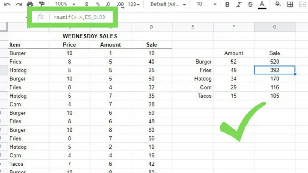
The sample dataset below is the Wednesday record of a food stall selling assorted snacks. I have four columns with headers: Item, Price, Amount, and Sale.
If I want to know how many burgers were sold I just need to modify the SUMIF Function syntax to reflect “=SUMIF(Item, “burger”, Amount)”.
What the SUMIF Function will do in this case is it will check the ‘Item’ column for rows that has the string “burger”.
In the same rows where the criterion is met, the SUMIF Function will get all the values from the ‘Amount’ column and add them up.
“=SUMIF(Item, “burger”, Amount)” can be further translated to “=SUMIF(A:A,”Burger”,C:C)” as the Item column is A:A and the Amount column is C:C.

This can also be done not just by putting in the exact criterion string but you can also use references to the cells containing your criterion.
This way, it’ll be easier to copy formulas down a list of items that you want to be summed up.
It’s also possible to have a single range be checked against the criterion and the ‘sum_range’ parameter as well as seen below where the 3rd optional parameter was skipped.
The result of the SUMIF Function, in this case, means that 68 orders of the total food sold number are from big orders alone.
This can be more significant when used in tandem with percentages, and other functions such as the COUNTIF Function.
Using the SUMIF Function with Blanks in Google Sheets
Another useful technique for the SUMIF Function in Google Sheets is to use it with blanks or non-blank specific cells in a dataset.
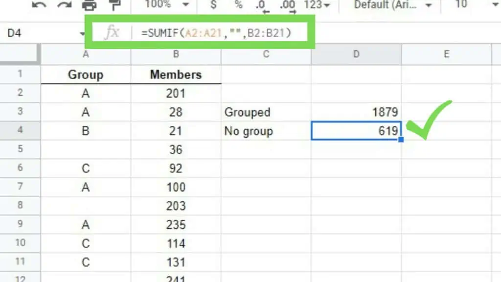
In the example dataset below, there were some groups that were assigned to larger groups: A, B, and C. That said, there were still some smaller groups that remained unassigned.
I want to see how many members belong to groups that were assigned to A, B, or C.
Using the sample below, the formula will be: “=SUMIF(A2:A21,”<>”,B2:B21)”.
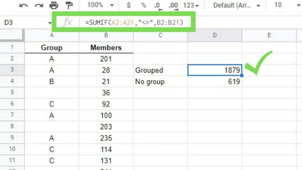
This means that using the “<>” criteria, which translates to “not equal to empty”, allowed the total number of “grouped” members to be computed.
Inversely, to compute the total number of “non-grouped” members, we just need to tweak the criterion to “” instead of “<>” – with the former meaning “empty” or “blank”.
Take note that the double quotes must be inputted without a space in between. Otherwise, it will be a criterion looking for values with a space.
The update formula will be: “=SUMIF(A2:A21,””,B2:B21)”.
Other than the usual operators such as greater than (“>”), less than (“<“), or equal to (“=”) – it’s great to know about the not equal to (“<>”), and empty signs (“”) as well.
Frequently Asked Questions about How to Use the Google Sheets SUMIF Function
Can I use multiple columns as the range for the SUMIF Function in Google Sheets?
The SUMIF Function in Google Sheets works for multiple cells, rows, and columns at the same time.As long as each value in that range meets the condition set, it will be added to the sum.
Can I use multiple criteria with the SUMIF Function in Google Sheets?
The SUMIF Function in Google Sheets only accepts one criterion and if you wish to use multiple criteria, use the SUMIFS Function instead. Its syntax is: SUMIFS(sum_range, criteria_range1, criterion1, [criteria_range2, criterion2, …]).
Conclusion on How to Use the Google Sheets SUMIF Function
To use the Google Sheets SUMIF Function, define a criterion and then identify the range to check against this criterion. Optionally, select a separate sum range for the return values. Lastly, use the formula: “=SUMIF(range, criterion, [sum_range])”.

