One of the common, if not the most used feature of Google Sheets is addition. Getting the sum of hundreds of numbers is easy.
I’ve been using the SUM Function for many years now, especially in cases where using the addition (+) operator is not sufficient.
In this tutorial, I’ll show you how to use Sum in Google Sheets.
How to Use Sum in Google Sheets
- Select an empty cell
- Type “=SUM(“
- Enter the range(s) or cells to add or press, hold, and drag over a range
- Type a closing bracket “)”
- Hit enter or click another cell

Using SUM in Google Sheets Video Tutorial
4 Different Ways to Use Sum in Google Sheets
The SUM Function is as simple as much as how useful it is. It returns the sum of a set of numbers and/or cells, and others depending on how you apply its parameter settings.
The syntax of the SUM Function is:
=SUM(value1, [value2, …])
Where each ‘value’ can be a number, cell, range, or even a function.
The values can refer to columns, rows, tables or matrices, or a combination of any of these.
1. Building The Sum By Using Columns
The most common way to use the SUM Function is by using columns as parameters.
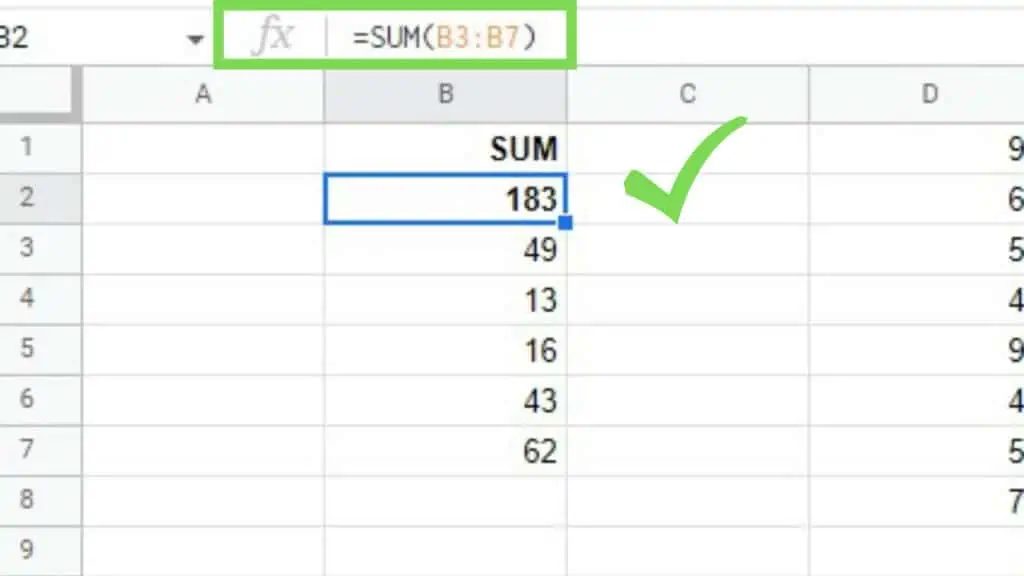
In the first example below, I’ve listed a small set of numbers arranged in a single short column.
The SUM Function is used here by simply using the whole range “B3:B7” as its value parameter.
Taking a different approach, I’ve created a longer set of numbers still arranged in a column. But this time, instead of identifying specific cell references, I simply pointed the SUM Function to the whole column “D:D”.
What this does is that literally every cell in that column will be taken in and added to the sum. If retroactively, I will add more numbers to column D, the SUM Function will be automatically updated to include the new number to the updated sum.

The only downside in using whole columns as the value for the SUM Function is that you cannot place your formula in the same column as it will result in a ‘circular dependency’ error.
2. Building A Sum By Using Rows
Since normally, we conduct the addition of larger numbers in a column fashion, using SUM for rows is not as common as the other one. That said, it’s still used quite often, especially for huge tables of data containing different categories of numerical values.
There’s not much difference in using SUM in Google Sheets for rows versus for columns – except that columns will give a vertical cell reference while rows give a horizontal reference.
In the next example, I created a small set of numbers arranged in a row.

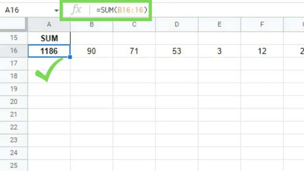
Similar to the example for columns, I also created a big set of numbers arranged covering a whole row except for its first cell where I’ve put the SUM Function.
Instead of using the whole row’s reference which is “16:16”, I instead used “B16:16”. This means that the value parameter will cover the whole row starting from B16 all the way to the rightmost cell.
Same with columns, the only downside in using whole rows as the value for the SUM Function is that you cannot place your formula in the same row as it will result in a ‘circular dependency’ error.
You can copy what I did in the last example though if you really want to put the SUM Function in the same row (or even column).
3. Building a Sumb by Using a Matrix in Google Sheets
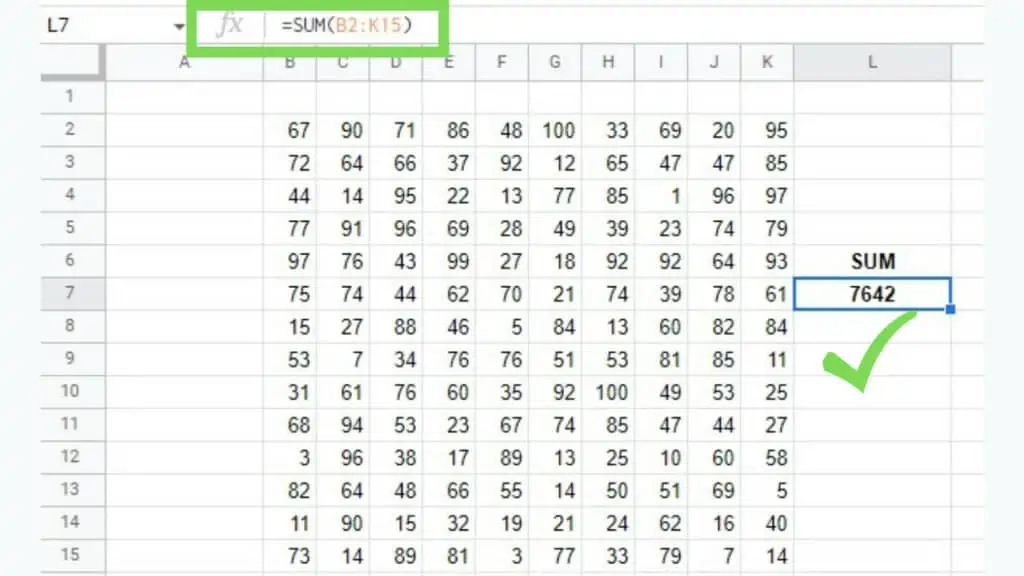
Another way to use SUM in Google Sheets is by using matrices or tables of numerical figures.
To do this, you can either manually type in the reference to the whole matrix or you can type in the first part of the formula [ =SUM( ] and then click on one corner and drag your mouse to populate the whole range.
This should automatically put the exact cell reference onto your formula.

Once done, the sum of all the numbers in the range that you have selected will be added together. If you edit any number within that range, the SUM Function will automatically update to calculate the new sum in Google Sheets.
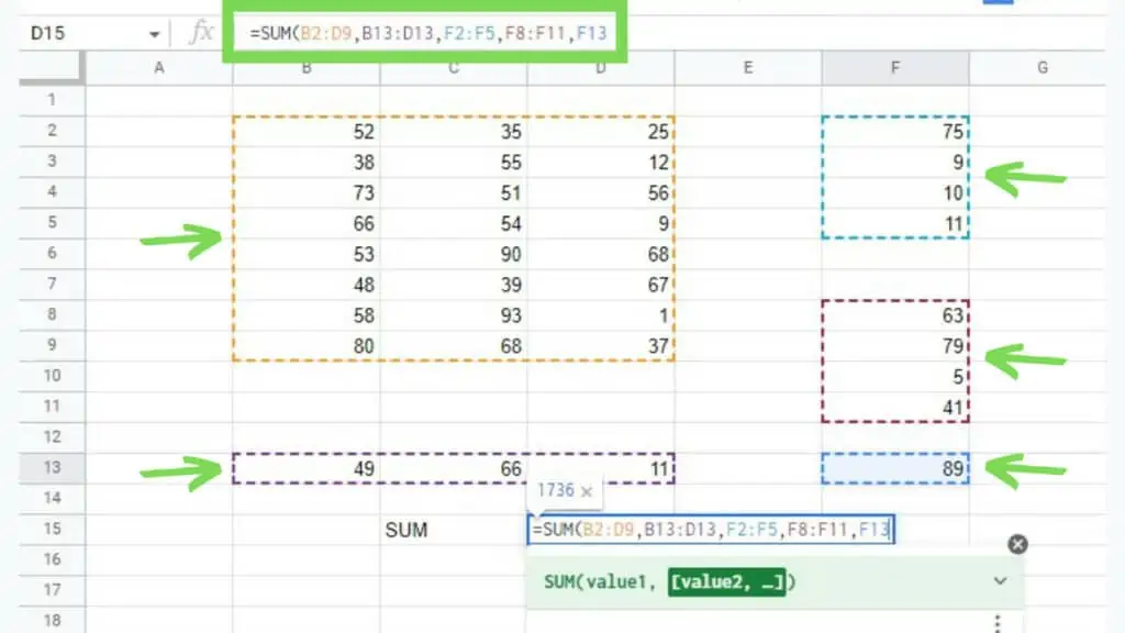
4. By Separate Ranges
Sometimes, your sheets are not arranged symmetrically and the numerical values that you wish to add will not be in a single row or column or may not even be adjacent to each other.
The great thing is that the SUM in Google Sheets can still calculate that as long as you input these ranges properly as the parameter of your SUM Function.
To do this, you may manually input each range’s cell reference into the SUM Function’s parameters – each separated by a comma.
An alternative way to do this, which is the one that I often use is to type in the first part of the formula which is [ =SUM( ], and then select your ranges one by one. Press and hold CTRL then start clicking and dragging your mouse to select those ranges.
They will be automatically populated and added in as value parameters to your SUM Function, each separated by a comma.
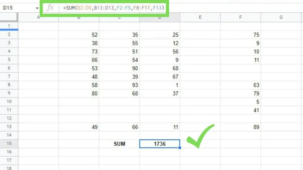
Either way, once you are done just hit enter or click on a different cell to display the results of Sum in Google Sheets.
Sum in Google Sheets is simple but is fundamental to a majority of use cases, especially in financial spreadsheets.
Other than addition, it is also important to know other operators such as for multiplication.
Frequently Asked Questions about How to Use Sum in Google Sheets
Can I use Sum in Google Sheets for datasets with negative numbers?
You can use Sum in Google Sheets for datasets with negative numbers by simply using them just like how you assign positive values to its parameters. The addition process will take note of their negative value and will subtract them from the sum instead of adding them.
Can I use Sum in Google Sheets to refer to the same cell more than once?
Sum in Google Sheets accepts the same cell as a reference even if it’s used twice or more. If a cell containing “1” is used thrice as a parameter for the SUM Function, it will add up to “3” instead of “1”.
Conclusion on How to Use Sum in Google Sheets
You can use SUM in Google Sheets by selecting an empty cell and typing “=SUM(“. Next, enter the range(s) or cells to be added or press, hold, and drag over a range. Afterward, type a closing bracket “)”. Lastly, hit enter or click another cell.

