
In this tutorial, I will teach you how to use ISBLANK in Google Sheets.
The ISBLANK function is an Info type of function that provides information on whether the cell or value referred to is blank, returning a TRUE if it is and FALSE if it is not.
And although it is commonly used in conjunction with the Logic types of functions to evaluate conditions, it can find some use where a boolean of TRUE or FALSE is needed.
It can even be used for Conditional formatting!
How to use ISBLANK in Google Sheets
To use the ISBLANK in Google Sheets write: “=IF(ISBLANK(A1),”This cell is blank”,A1)”. Substitute A1 with the corresponding cell address.
ISBLANK Function Syntax Explained
ISBLANK(value)
- value: a value, formula, or reference to a cell that is evaluated to be blank or not
Methods For ISBLANK Function
For this tutorial, it is important to know whether the ISBLANK function returns as a blank or not:
White spaces (“ ”), empty strings (“=”””), new lines (“=CHAR(10)”), and errors could be misconstrued as blanks for values, but the ISBLANK function returns FALSE for these values.
And aside from a literal cell without a value in it, only the =IFERROR(0/0), even if it is a formula, returns TRUE.
Using this information, you can create a range of values with non-blank cells and an assortment of the different values that return TRUE to test out some of the methods I will teach you.
Method 1 – Identify blank cells within a range
For this method, please populate a column with an assortment of white spaces, empty strings, new lines, values, and blanks to apply a formula on.
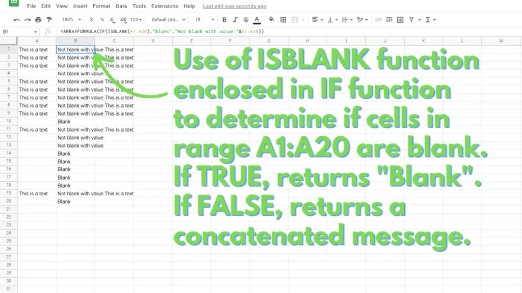
Assuming that the column filled is column A, and the range address is A1:A20, substitute this address on the [range address] part of this formula, then paste it on cell B1:
=ARRAYFORMULA(IF(ISBLANK([range address]),”Blank”,”Not blank with value:”&CHAR(10)&[range_address]))
For context, the formula repeats an IF function that checks whether the cell, from A1:A20, is blank. If it is blank according to the ISBLANK function, then the text “Blank” is returned.
If not, then an appended text containing “Not blank with: ”, then the content of the non-blank cell is displayed.
This is how it should look like:
Method 2 – Identify addresses of blank cells within a range
For this method, you can keep using the range that you referred to for Method 1.
Given the results of Method 1, you now have an idea where the blank cells are, so you would be able to check the veracity of the formula for this method:
=FILTER(
ARRAYFORMULA(IF(ISBLANK([range address]),”[column letter]”&ROW([range address]),IFERROR(0/0))),
ARRAYFORMULA(IF(ISBLANK([range address]),”[column letter]”&ROW([range address]),IFERROR(0/0)))<>””)
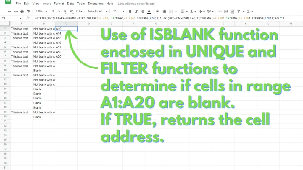
Just like on method 1, simply substitute your range address onto the [range address] part of the formula, substitute the column letter for your range onto [column letter], then paste it on cell C1 of your worksheet.
This formula is very similar to the formula for method 1, with an added filter that removes blank results, ending up with a list-like result.
For context, the formula repeatedly checks the [range address] to see if it is blank, and if it is, an appended message consisting of [column letter] and the row of the blank cell is returned.
If not, a blank cell is returned.
It is then filtered to remove blank cells, leaving you with a list-like result of the addresses of the blank cells.
The result should look like this:
Method 3 – Count blank cells within a range
For this method, you can keep using the initial range that was referred to in the previous methods.
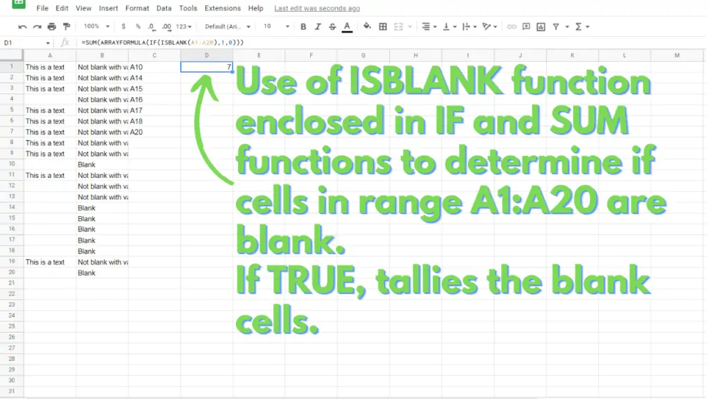
Substitute your range address to range address of this formula, then paste it on cell D1 of your worksheet:
=SUM(ARRAYFORMULA(IF(ISBLANK([range address]),1,0)))
The formula repeatedly checks each cell in your range for blank cells, and if a cell is blank, the value 1 is returned, while the value 0 is returned if it is not blank.
This section is then enclosed by a SUM function that adds all the 1 values, essentially tallying how many blank cells there are in the range.
The result should look like this:
Read about how to use the IF function next.
ISBLANK Function in Google Sheets Examples:
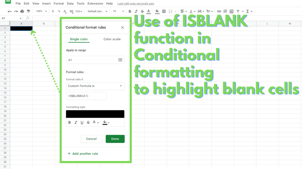
Custom Conditional Formatting Formula that highlights cell A1 in black if it is blank:
=ISBLANK(A1)
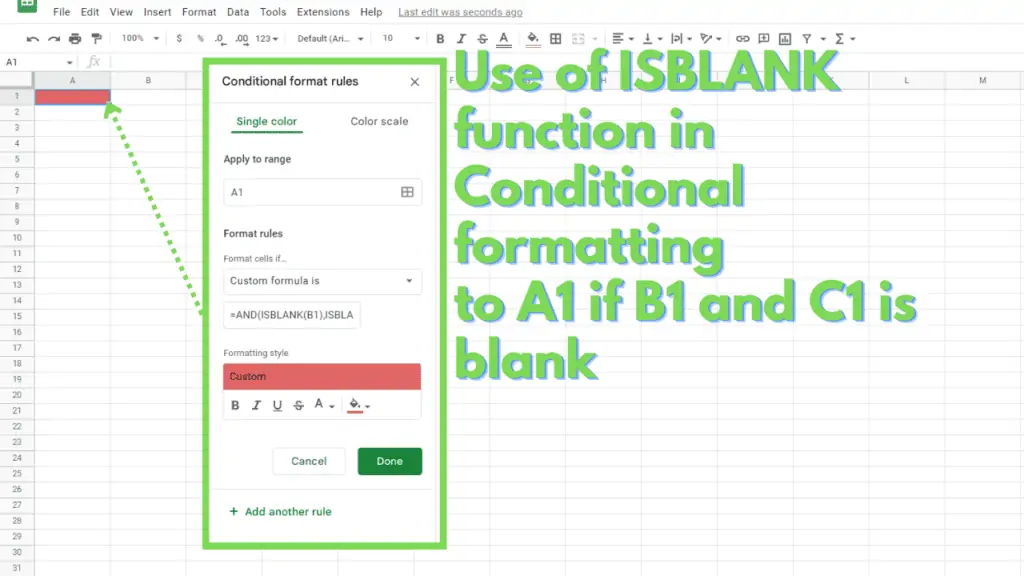
Custom Conditional Formatting Formula that highlights cell A1 in red if cells B1 and C1 are blank:
=AND(ISBLANK(B1), ISBLANK(C1))
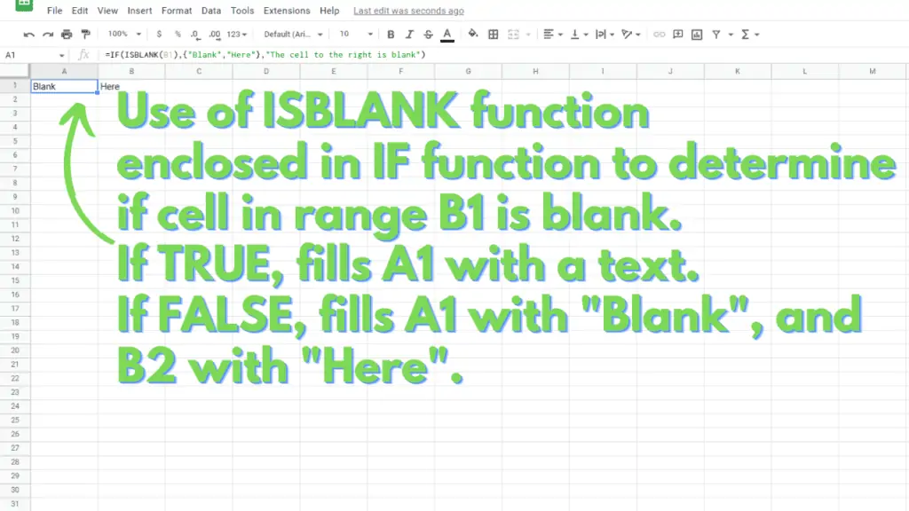
Formula on A1 that checks if cell B1 is blank, and if it is, displays texts “Blank” and “Here” in A1 and B1, respectively through an array. If not, display “The cell to the right is blank”:
=IF(ISBLANK(B1),{“Blank”,”Here”},”The cell to the right is blank”)
Frequently Asked Questions on How to Use the ISBLANK Function in Google Sheets
How do I use the ISBLANK function in Google Sheets?
The ISBLANK function itself is a simple function that checks whether value or cell reference is blank. The syntax is “ISBLANK(value)”, where value is either a value itself or a cell reference. The ISBLANK function returns TRUE if the value is blank, and FALSE if it is not. It is commonly used in conjunction with the IF function or any function that accepts TRUE or FALSE as an argument.
The “” output of my formula is not being evaluated as TRUE by the ISBLANK function, can I use something else as output in Google Sheets?
The syntax “” is referred to as an empty string and is not considered a blank. You can use IFERROR(0/0) instead, as it is considered a blank by the ISBLANK function.
Can I use the ISBLANK function to check if 2 or more cells are blank at the same time in Google Sheets?
You can use the AND Logical function for this purpose. The syntax would be:
=AND(ISBLANK(cell 1),ISBLANK(cell 2)). Simply substitute the address of your 2 cells as cell 1 and cell 2, respectively.
Conclusion on how to use the ISBLANK function in Google Sheets
To use the ISBLANK function as a condition for formulas that perform actions depending on the blank state of a cell or value use:
“=IF(ISBLANK(A1),”This cell is blank”,A1)”
Substitute both instances of A1 with the address of the cell that you want to evaluate.

