
In this tutorial, I will explain how to use IMPORTRANGE in Google Sheets.
Often, Google Sheets users want to set up connections between Google Sheets files.
For most cases, simply copying and pasting a range of entries from one file to another will suffice.
However, that method is not scalable and it is time-consuming and manual. For scalability and automation, the IMPORTRANGE function will allow you to automatically import data from a different file to your current file.
The data can be in the form of raw data, tables, pivot tables, etc. As long as the value to import is stored in cells, the IMPORTRANGE function can import it.
And, because the imported data is laid out in cells, you are free to process them further with the use of Pivot Charts or Pivot Queries.
How to use IMPORTRANGE in Google Sheets
To use IMPORTRANGE in Google Sheets, follow these steps:
- Identify the file, sheet name, and range that you will import data from
- Make sure that you have access to the file you will import data from
- Construct the IMPORTRANGE formula using the source file link, sheet and range:
“=IMPORTRANGE([Source file link],[Sheet name]![Range])”
Using Importrange in Google Sheets Video Tutorial
How to Import Data from a different Sheet in Google Sheets
For this tutorial, I will provide a sample file that has 3 sheets.
The first sheet will contain values that simulate raw data, while the second and third sheets will contain tables and pivot tables derived from the raw data of the first sheet.
We will be using a copy of this file, with a file of your own, to import the raw data and tables.
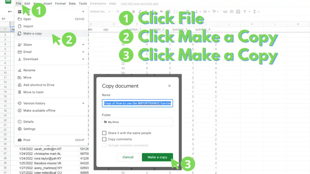
You can make a copy of the file by accessing it through this link, then click on “File” from the Menu Bar, and select “Make a copy”.
A dialog box appears. Within it, you can provide a filename for the Copy then click “Make a Copy”.
Step 1 – Identify the link and the range for the source of your IMPORTRANGE
The syntax for the IMPORTRANGE function that we will use is as follows:
=IMPORTRANGE([Spreadsheet URL],[Range String])
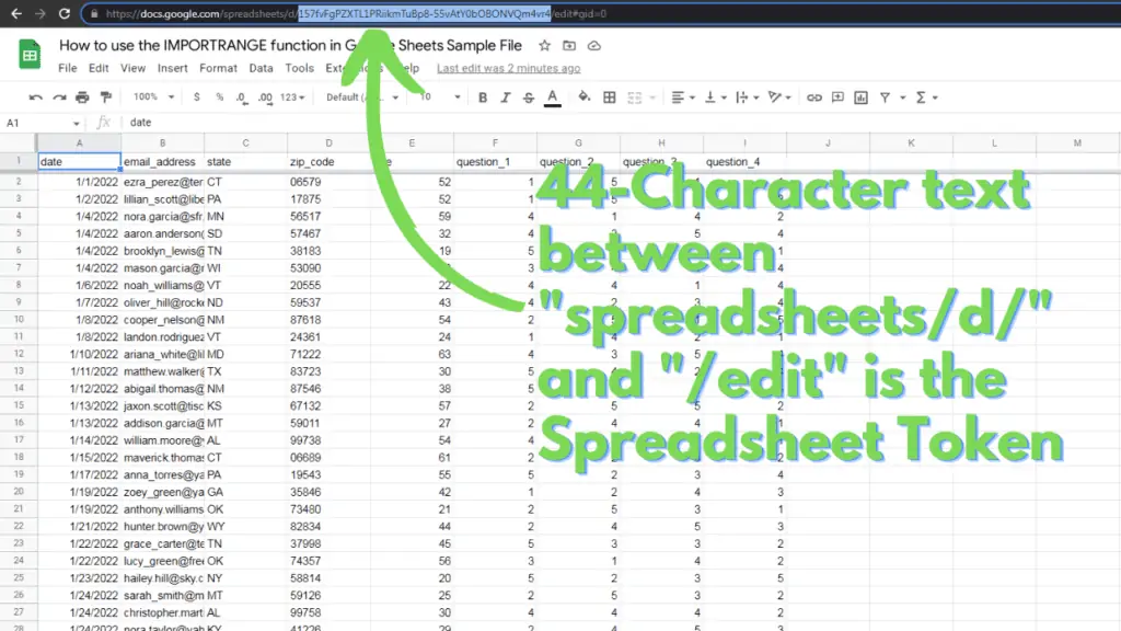
The spreadsheet URL section accepts a Google Sheets link.
It can be found in the address bar whenever you have the Google Sheets file open.

Alternatively, this section will work with the Google Sheets token of the Spreadsheet URL.
The token of a spreadsheet URL is the 44-character string between “/spreadsheets/d/” and the next “/edit”.
The range string section will need to be filled with a string using the following syntax:
=IMPORTRANGE([Spreadsheet URL],[Sheet Name]![Range Address])
As an example, the range string for data in Sheet3 cells A1 to B5 is:
=IMPORTRANGE([Spreadsheet URL],Sheet3!A1:5)
Take note of how to identify [Spreadsheet URL], [Spreadsheet Token], and [Range String], as you will need them to modify the IMPORTRANGE function according to what you need to import.
Step 2 – Ensure that you have access to the source file
To secure the Data for Google Sheets users, the IMPORTRANGE function cannot import data from a file that users do not have access.
To get around this, either make sure that you’re importing from a file that you own or request access to the file you want to use.
Only view access is needed for the IMPORTRANGE function to work.
To confirm whether you have access to the file, try to open it through its link.
If you don’t have access to the file, you will be redirected to a page like this:

Step 3 – Construct the IMPORTRANGE Formula
Now that you have the prerequisites, a copy of the source file that you own with its link or token, and a destination file, we can now create the IMPORTRANGE formulas.
In your destination file, prepare two blank sheets.
You should already have one by default, but to create blank sheets, simply click on the “Plus” sign at the bottom left part of Google Sheets.

For all of the formulas, we will discuss, you should use a different [Source File Link] from the examples.
On the first blank sheet, we will create an IMPORTRANGE formula to transfer data from the Raw Data sheet.
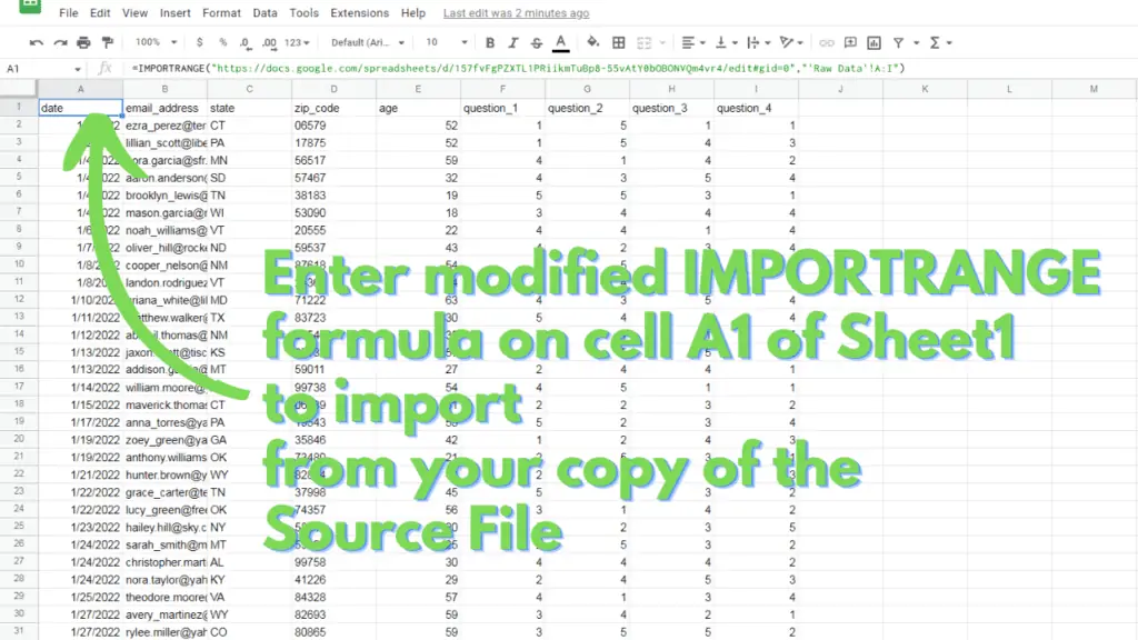
Modify this formula by replacing [Source File Link] with either the spreadsheet URL or spreadsheet token of the source file, [Sheet Name] with the sheet name of the source file (“‘Raw Data’”), then [Range] with the range address that you want to import (“A1:I102” or “A:I”).
=IMPORTRANGE([Source File Link],[Sheet Name]![Range])
After you’ve modified it, paste the resulting formula on cell A1 of your first blank sheet.
Usually, the first IMPORTRANGE from a new Source File applied on a sheet will prompt you to allow or deny the formula access.
This is implemented for security purposes. If you encounter this, simply hover over the cell where the formula is and click “Allow Access”.
After pasting the formula and allowing it to access the Source File, the result should look like this:
On the second blank sheet, we will now create an IMPORTRANGE formula to transfer tables from the Tables and Pivot Tables sheet.
For this, we need a minimum of two IMPORTRANGE formulas.
Modify the first of the two formulas by replacing [Source File Link] with either the link or token of the source file, [Sheet Name] with the sheet name of the source file (“Tables”), then [Range] with the range address that you want to import (“A1:D5”).
After you’ve modified it, paste the resulting formula on cell A1 of your second blank sheet.
The formula and result should look like this:

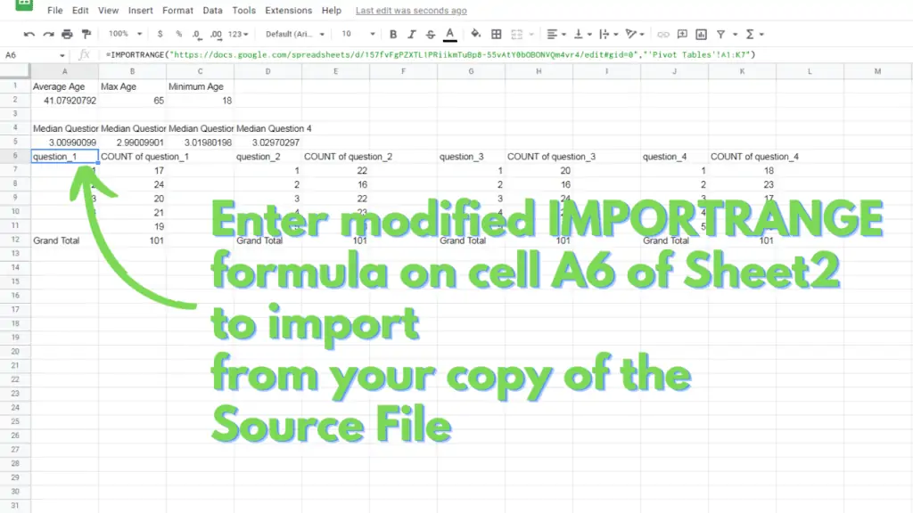
Finally, modify this formula by replacing [Source File Link] with either the link or token of the source file, [Sheet Name] with the sheet name of the source file (“’Pivot Tables’”), then [Range] with the range address that you want to import (“A1:K7”).
After you’ve modified it, paste the resulting formula on cell A6 of your second blank sheet.
The formula and result should look like this:
You now know How to use the IMPORTRANGE function in Google Sheets!
Frequently Asked Question on How to use IMPORTRANGE in Google Sheets
Is there a limit on how many cells the IMPORTRANGE function can import into Google Sheets?
There is a hard limit on how many Cells a spreadsheet file can have, this is set to 10 million cells. The closer one is to this limit, the slower the file will function. Through my experience, though, IMPORTRANGE usually fails at around 600,000 cells from a single file, or 20,000 rows by 30 columns. Even dividing the import by 2, using 2 IMPORTRANGE functions to import 300,000 cells each, does not fix this.
Can I use IMPORTRANGE to import a chart from another file in Google Sheets?
Unfortunately, the IMPORTRANGE function can only import data stored in cells. Charts are objects independent from cells, and as such, cannot be imported through the IMPORTRANGE function.
Conclusion on How to use IMPORTRANGE in Google Sheets
To use IMPORTRANGE in Google Sheets identify the link of the Google Sheets file that you will import from. You can use the link directly, or it’s Token. The Token is composed of 44 characters directly after “/spreadsheets/d/” in the link for a Google Sheets file.
Next, make sure that you have access to the Source File, even View access will be enough for the IMPORTRANGE function to work.
Finally, modify the IMPORTRANGE formula
=IMPORTRANGE([Source File Link],[Sheet Name]![Range])
Replace [Source File Link] with either the link of the file, or the Token within the link, then replace [Sheet Name] with the worksheet name (“Sheet1”, “Sheet2”, etc.), then replace [Range] with the range of the cells that you will import (“A1”, “A1:C100”, “A:C”).
Once the formula has been finalized, enter it in a cell of your choice in the Destination file.

