In this tutorial, I will teach you how to use Google Sheets Query label.
The Query function is Google Sheet’s implementation of SQL (Structured Query Language).
SQL is a programming language that allows you to perform processes on relational data, like aggregating totals, defining averages, arriving at differences, etc.
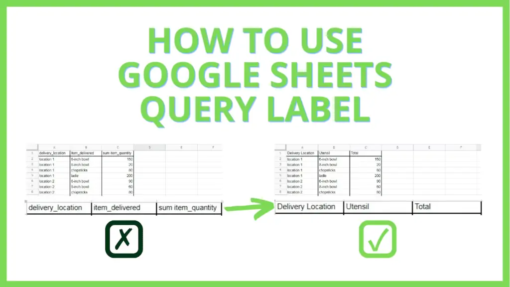
However, you will notice that column headers produced by Query are generated depending on the process the query applied.
A column summation will appear as “sum [column header]” or “sum(col1)”.
While this may not be a problem for most situations, there are times when renaming the resulting column header is needed. In those situations, the Google Sheets Query Label is exactly what you need.
How to use Google Sheets Query Label:
To use the Google Sheets Query Label:
- Add Data to Google Sheet
- Create a new Tab
- Apply a simple Query function on cell A1 of the new Tab. Example: =QUERY(Sheet1!A:E,”SELECT B, C, SUM(D) WHERE B IS NOT NULL GROUP BY B, C”)
- Identify the resulting column header that you will change
- Edit the Query function and apply the Query Label in the Query String
Use Query Labels in Google Sheets Video Tutorial
How to use Google Sheets Query Label – Step by Step
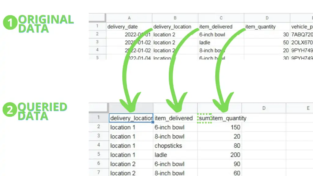
For this tutorial, we will be using a dataset that represents inventory deliveries to several locations.
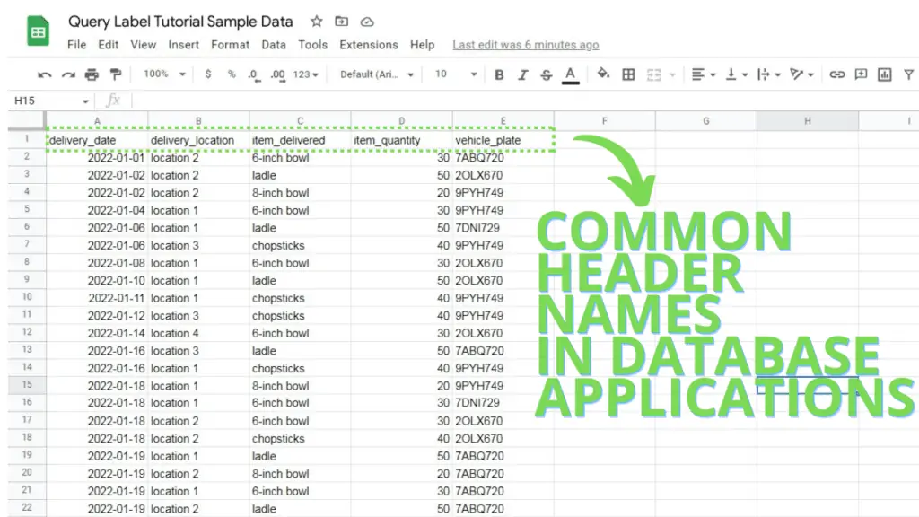
You may notice that the column headers I provided use underscores instead of spaces, and are all in lowercase.
This is to simulate an “exported” data file from common database applications.
Step 1 – Add Data to Google Sheet
Before starting on learning how to use Google Sheets Query Labels to change the column headers, we need to have a dataset that we will process with the Query function.
On that front, I created a simple dataset for us to process through this file.
You can go ahead and copy the data to be pasted on a different Google Sheets file,
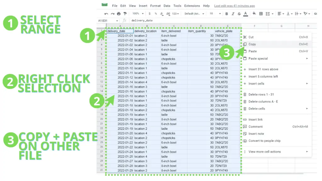
or duplicate it directly by clicking ‘Make a Copy’ under the ‘File’ tab.
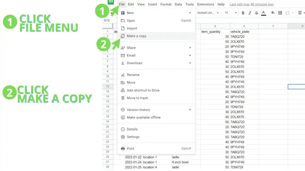
If you opted to paste the data on a different Google Sheets file, make sure that the Tab name that you pasted it on is “Sheet1”, the default Tab name for the first tab in all Google Sheets files.
This is important as the formula we will use later will reference the data from the “Sheet1” tab.
Step 2 – Create a new Tab
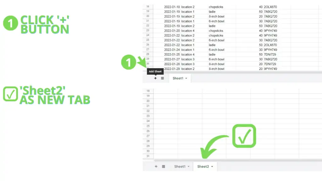
On the Google Sheets files that you either pasted the data to or duplicated from the file I provided, create a new Tab by clicking the ‘Plus’ button at the lower left-hand corner of Google Sheets. By default, this new tab should be named ‘Sheet2’.
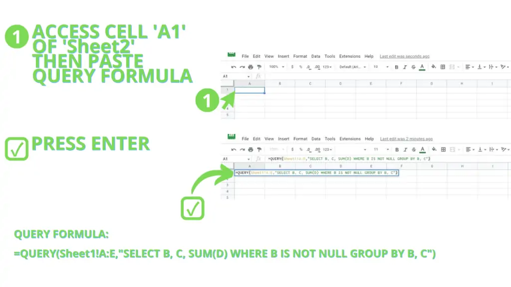
Step 3 – Apply a simple Query function on cell A1 of the new Tab
=QUERY(Sheet1!A:E,”SELECT B, C, SUM(D) WHERE B IS NOT NULL GROUP BY B, C”)
The Query function should generate a table that looks like this:
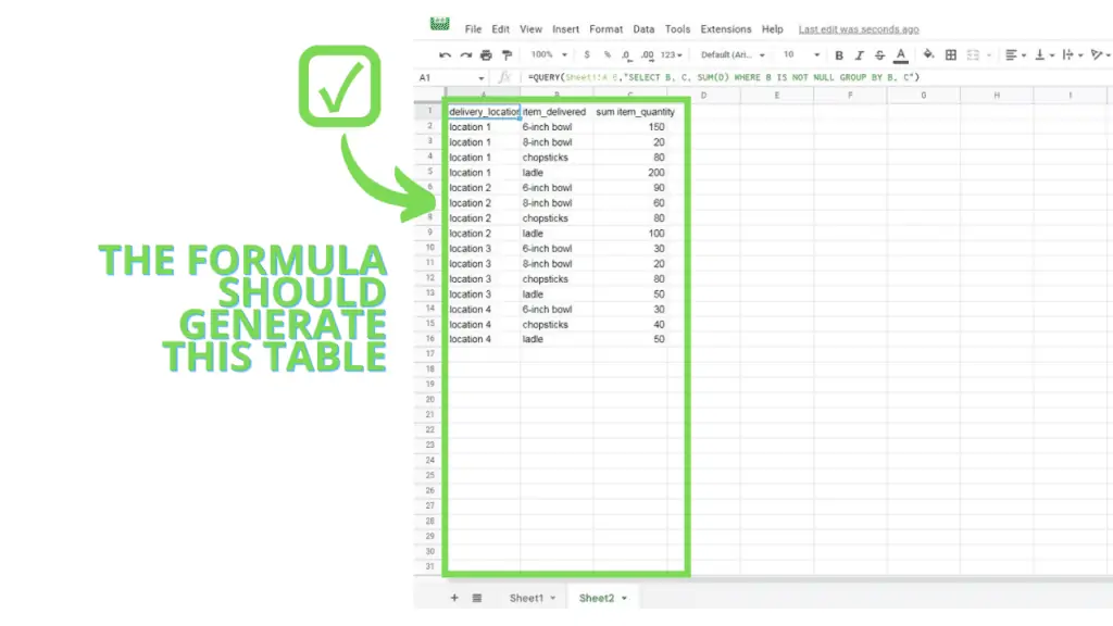
Step 4 – Identify the resulting column header that you will change
As you can see on the Query generated table, the column headers have been retained from the dataset, apart from one which was a result of a Math operation from our Query, “SUM(D)” to be precise.
The resulting column header’s syntax for our example is the operation (sum), a space separator, and the column header that the operation was applied on. Hence, “sum item_quantity”.
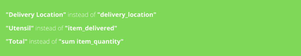
Let’s assume that we need to change these column headers from being programmatic to something more organic: Delivery Location instead of delivery_location, Utensil instead of item_delivered, and Total instead of sum item_quantity.
From our Query string of “SELECT B, C, SUM(D) WHERE B IS NOT NULL GROUP BY B, C”, we can identify the following:
- delivery_location is B
- Item_delivered is C
- sum item_quantity is SUM(D)
Keep these in mind when we edit the Query to rename the Query Labels or resulting column headers.
Step 5 – Edit the Query function and apply the Query Label in the Query String
Now that we have identified the column headers that we want to change through the Google Sheets Query Label, our next and final step is to learn how to write a Query Label and where to put it in the existing Query function.
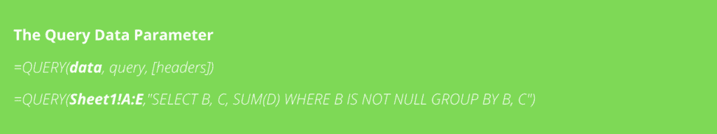
This is the structure of the Query Function:

=QUERY(data, query, [headers])
1. The ‘data’ parameter is used to refer to a range that the Query function will process. From the Query function that we’re using, this would be Sheet1!A:E, or columns A to E of a tab with Sheet1 as its name
2. The ‘query’ parameter is where the query string is placed. We can describe it as a string for a command that will tell Google Sheets which columns to process, what processes to apply, what organization to apply to which columns, in what order to list the results, etc.
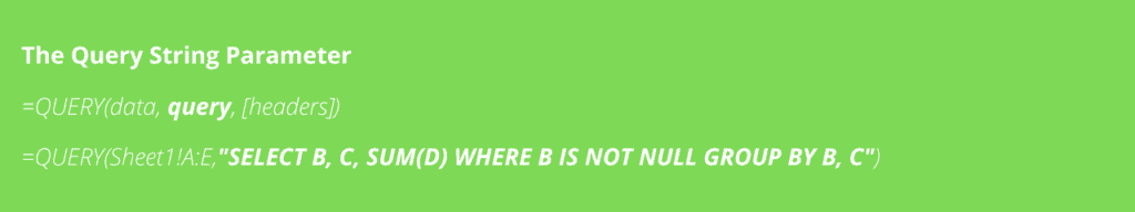
From the Query function that we’re using, this would be “SELECT B, C, SUM(D) WHERE B IS NOT NULL GROUP BY B, C”. To describe what the query string does, we have to look at its parts.
The “SELECT B, C, SUM(D)” is what’s called the Select clause. This part tells Google Sheets which columns to process, and what operation to apply. If you only want to show the contents of the column, you don’t need to add an operation like SUM.

The “WHERE B IS NOT NULL” is what’s called the WHERE or Condition clause. This part tells Google Sheets the conditions to apply on the columns that were selected. The ‘WHERE’ word indicates the start of the Condition clause.

In this case, the condition that we want is to be able to process the Select clause (column B, column c, the sum of column D), but only on items where column B is not blank, hence ‘WHERE B IS NOT NULL’.
The last part of our query string is what’s called the Group by clause.
This allows us to tell Google Sheets how we want the resulting data to be grouped. The ‘GROUP BY’ words indicate the start of the Group by clause.

In this case, then, we want Google Sheets to group the results first by column B, then next by column C.
3. The last parameter of the Query function, the ‘headers’ parameter, is an optional one. This allows us to set how many rows from the dataset will be considered as ‘headers’, and thus be excluded from any operations by the different clauses.
Leaving it blank, like in our case, leaves Google Sheets to scan our data to automatically identify how many rows it will consider as header rows.

Now that we know the different parameters of the Query function, together with the different clauses of the query string, we’re ready to learn how to use Google Sheets Query Label to rename column headers.
Incidentally, like the different clauses of a query string, the Google Sheets Query Label is also its own separate clause: the Label clause. The start of the Label clause is indicated by ‘LABEL’.
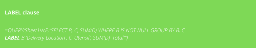
Its syntax is similar to the other clauses as shown below,

with the starting point indicator, and resulting header column identifier. The only difference is how we introduce the name that we would like to replace the generated column name with.
The syntax starts with “LABEL”, followed by the column to be changed, followed by what we’d like to change it into enclosed by 2 apostrophes (‘), then a comma to separate each successive label change.
In the case we’ve discussed back in Step 4, we will change column B, C, and SUM(D) to be named Delivery Location, Utensil, and Total, respectively.
To change column B to ‘Delivery Location’, part of the Label clause would look like this:
“B ‘Delivery Location’”
To change column C to ‘Utensils’, part of the Label clause would look like this:
“, C ‘Utensils’”
Finally, to change column SUM(D) to ‘Total’, part of the Label clause would look like this:
“, SUM(D) ‘Total’”

You will need to combine the indicator for the Label clause, “LABEL”, with these 3 parts, then add them at the end of the query string to apply a Query Label change.
The final Label clause should look like this:
“LABEL B ‘Delivery Location’, C ’Utensils’, SUM(D) ‘Total’”.

Now, this final Label clause is what we will add at the end of our current query string. Once added the query string should be as follows:
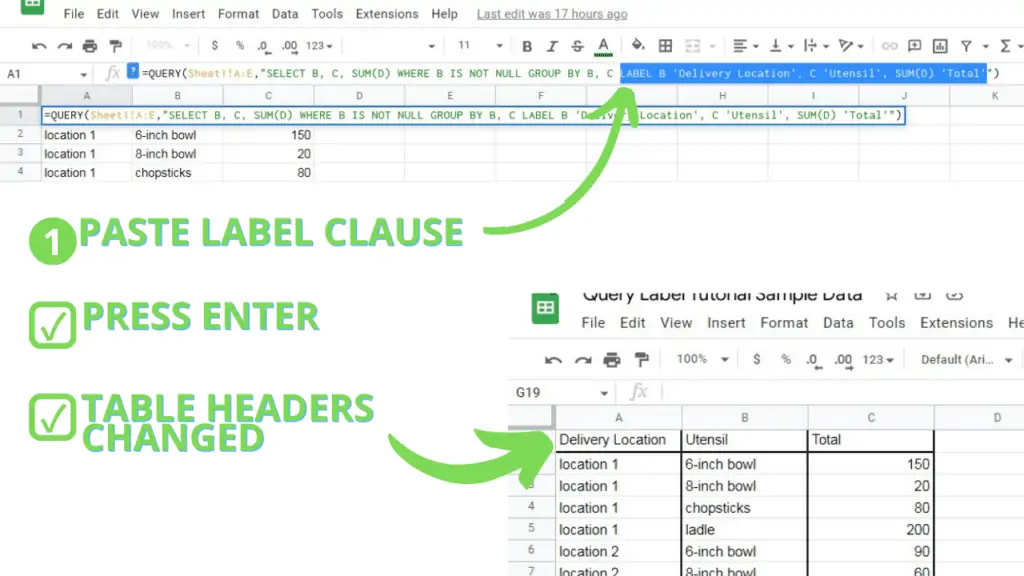
“SELECT B, C, SUM(D) WHERE B IS NOT NULL GROUP BY B, C LABEL B ‘Delivery Location’, C ‘Utensil’, SUM(D) ‘Total’”
Once you’ve added the Query clause, hit Enter to confirm the changes we made on the Query parameter of the Query Function. The resulting table should now carry the changes we instructed Google Sheets to apply to the column headers, and should look like this:
Frequently asked Questions on How to use Google Sheets Query Label
Is there a character limit on the column header that I want to replace an existing one with in Google Sheets?
There is no limit on the length of the new column header, but it’s best practice to keep it short and simple, and to make sure that it fits nicely into the size of the column.
How can I apply formatting to a created table in Google Sheets?
You can apply formatting to the resulting table, whether it’s just for the column headers or the resulting data, through the usual formatting options provided by Google Sheets.
Will changing my raw data’s headers mess with the changes from the Query Label in Google Sheets?
The Label clause of the Query string identifies the header to be changed from either its column name and operation (A, SUM(B), AVG(C), etc), or index in an array (Col1, SUM(Col2), AVG(Col3)), and is independent of its contents.
Therefore, no changes will be applied to the final table if the source column headers’ contents are changed.
Conclusion on How to use Google Sheets Query Label
To use Google Sheets Query Label add what’s called a Label clause on the Query parameter of a Query function. First, you identify which headers you need to change and what to change them into. Next, you finalize and combine the changes you want to make into a Label Clause that you will paste on the Query String of your Query function.

