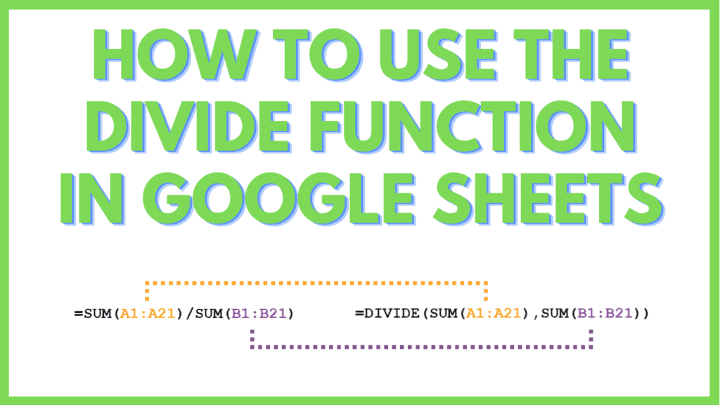
In this tutorial, I will show you how to use DIVIDE in Google Sheets.
The DIVIDE function is an Operator function that translates the commonly used divide operator “/” into a formula. Similar to how the MULTIPLY Operator is “*” in the Google Sheets multiplication function.
DIVIDE Function in Google Sheets Syntax
DIVIDE(dividend, divisor)
How to Use DIVIDE in Google Sheets:
- Divide the numbers in a column by a single number by using and copying the formula =DIVIDE([column_range], [number]) down a column
- Divide a single number by the numbers in a column by using and copying the formula =DIVIDE([number], [column_range]) down a column
- Divide the numbers in a column by the numbers in a different column by using and copying the formula = DIVIDE([dividend_range], [divisor_range]) down a column
- Improve the readability of complex formula
ARRAYFORMULA(IF(A2:A=””,””,A2:A/ARRAY_CONSTRAIN(TRANSPOSE(SPLIT(REPT(“21|22|23|”,100),”|”,1,0)),21,1)))
through the use of a DIVIDE function to turn it into
=ARRAYFORMULA(IF(A2:A=””,””,DIVIDE(A2:A,ARRAY_CONSTRAIN(TRANSPOSE(SPLIT(REPT(“21|22|23|”,100),”|”,1,0)),21,1))))
Divide in Google Sheets Video Tutorial (Step-By-Step)
How DIVIDE Works
Within this DIVIDE formula are 2 required parameters called [dividend] and [divisor], where the [dividend] is the number to be divided, and the [divisor] is the number to divide the dividend with.
Operator functions like DIVIDE are usually used to improve the readability of very complex formulas, where it can prove difficult to identify which parts of a formula constitute the dividend or the divisor.
The DIVIDE Function Syntax for Google Sheets Explained
DIVIDE(dividend, divisor)
- dividend: The number to be divided by the divisor
- divisor: The number to divide the dividend by, cannot be a zero
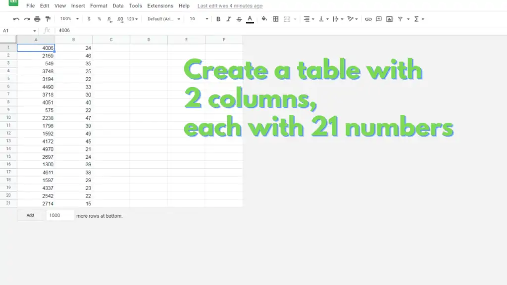
For this tutorial, you will need values across 2 columns to use for the DIVIDE function.
On both columns, please provide numbers for 21 rows where the second column does not contain a zero.
Once done, your table should have 2 columns and 21 rows as its dimension, and should look like this:
DIVIDE in Google Sheets Methods
Method 1 – Divide the numbers in a column by a single number by using and copying the formula =DIVIDE(dividend, divisor) down a column
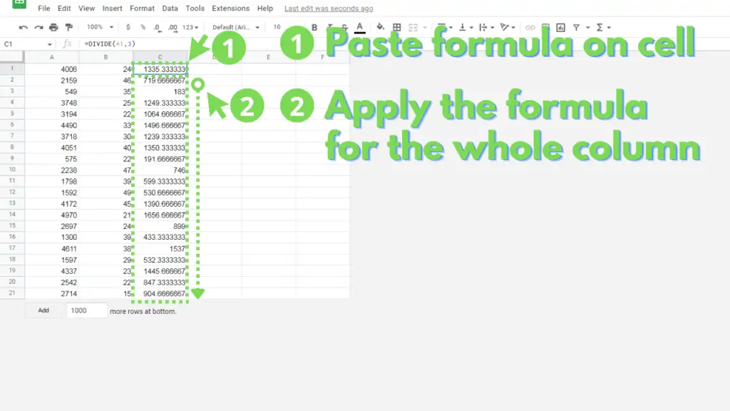
For this method substitute the dividend with the address of a cell. Use cell A1 from the table you created for our example. Then, substitute the divisor with any non-zero number. Use 3 for our example. The formula should look like this:
=DIVIDE(A1, 3)
Enter this formula on cell C1, then copy and paste it from cell C2 to cell C21. Your table should now look like this:
Method 2 – Divide a single number by the numbers in a column by using and copying the formula =DIVIDE([number], [column_range]) down a column
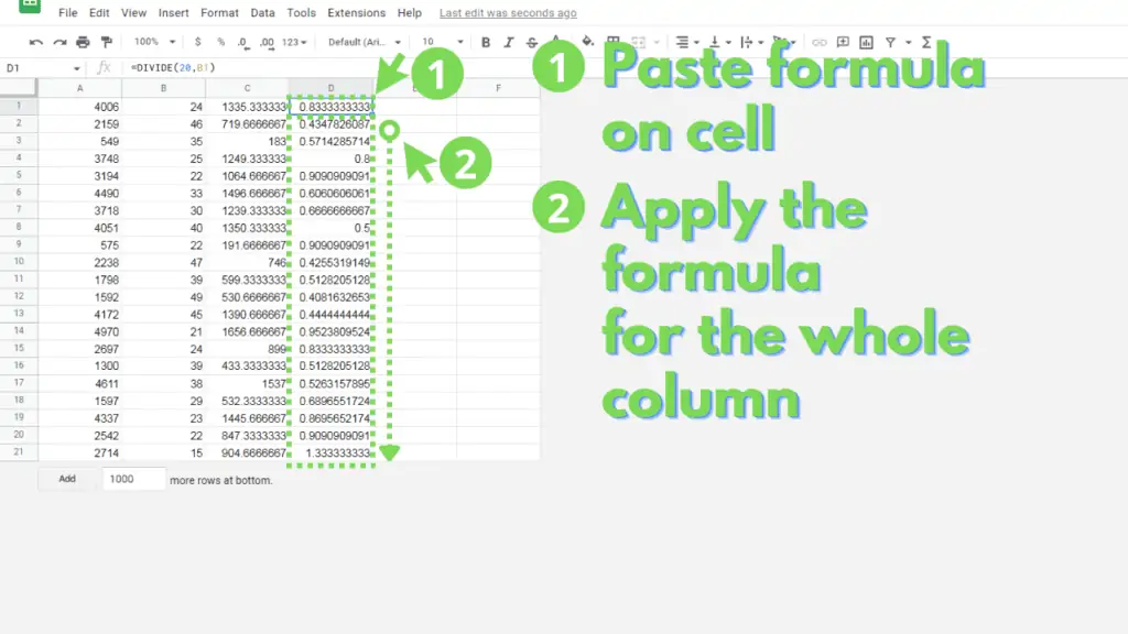
For this method, substitute the dividend with a single number. Use 20 for our example. Then, substitute the divisor with the address of a cell. Use cell B1 from the table you created for our example. The formula should look like this:
=DIVIDE(20, B1)
Enter this formula on cell D1, then copy and paste it from cell D2 to cell D21. Your table should now look like this:
Method 3 – Divide the numbers in a column by the numbers in a different column by using and copying the formula =DIVIDE([dividend_range], [divisor_range]) down a column
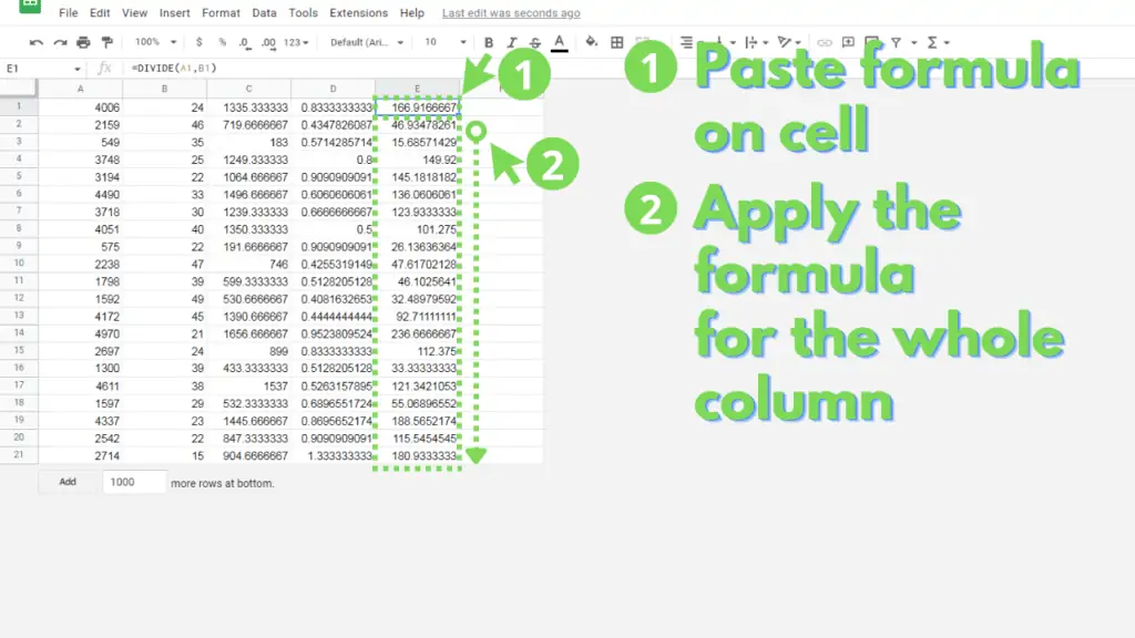
For this method, substitute the dividend with the address of a cell. Use cell A1 from the table you created for our example. Then, substitute the divisor with the address of a cell. Use cell B1 from the table you created for our example. The formula should look like this:
=DIVIDE(A1, B1)
Enter this formula on cell E1, then copy and paste it from cell E2 to cell E21. Your table should now look like this:
Method 4 – Improve readability of complex formula through the use of a DIVIDE function
For this method, you will improve the readability of a complex formula by using the DIVIDE function instead of the divide operation “/”.
The formula we will convert is:
=ARRAYFORMULA(IF(A1:A=””,””,A1:A/ARRAY_CONSTRAIN(
TRANSPOSE(SPLIT(REPT(“21|22|23|”,100),”|”,1,0)),21,1)))
You can identify the second instance of A1:A as the dividend, and the following as the divisor:
ARRAY_CONSTRAIN(TRANSPOSE(SPLIT(REPT(
“21|22|23|”,100),”|”,1,0)),21,1)
You can then substitute A1:A as the dividend, then the subpart of the formula as the divisor to arrive at this formula:
=ARRAYFORMULA(IF(A1:A=””,””,DIVIDE(A1:A,ARRAY_CONSTRAIN(TRANSPOSE(SPLIT(REPT(“21|22|23|”,100),”|”,1,0)),21,1))))
Paste this formula on cell F1. After which, your table should now look like this:
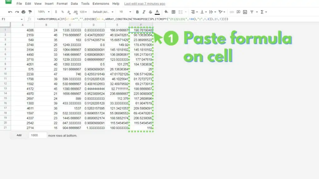
For context, the formula will check the presence of a value from A1 to A21, then, if a value is present, divide it by seven instances of the sequence 21,22, and 23 (4006/21, 2159/22, 549/23, 3746/21, 3194/22, etc.).
Frequently Asked Questions on How to use DIVIDE in Google Sheets
How do I use the DIVIDE Function in Google Sheets?
Using the formula =DIVIDE(dividend, divisor), substitute dividend with either a number or a cell address, then substitute divisor with either a non-zero number or a cell address.
Is the DIVIDE function the same as the QUOTIENT function in Google Sheets?
The QUOTIENT function divides a dividend by a divisor and returns a result without its remainder (if any), while the DIVIDE function returns a result with a remainder (if any) in the form of a decimal.
Can the DIVIDE function return an array of results without the use of ARRAYFORMULA in Google Sheets?
The DIVIDE function can only use a single cell or number for both its dividend and divisor, thus only returning a single result. The ARRAYFORMULA function essentially repeats a function across a range of cells, returning an array of results.
Divide Function in Google Sheets Examples
Use DIVIDE to divide 10 by 2:
=DIVIDE(10, 2)
Use DIVIDE to divide cell A20 of current sheet by cell A20 of Sheet1:
=DIVIDE(A20, Sheet1!A20)
Use DIVIDE to divide 300 with cell C1 of Sheet3:
=DIVIDE(300, Sheet3!C1)
Conclusion on How to use DIVIDE in Google Sheets
There are several common uses for the DIVIDE function.
First, you can divide the numbers in column A by a single number by replacing [dividend] with cell A1, then the [divisor] with a non-zero number for the formula =DIVIDE([dividend], [divisor]). Next, copy and paste the formula to the subsequent cells from your result.
Next, you can divide a single number by non-zero numbers in a column by replacing [dividend] with a number, then the [divisor] with cell B1 for the formula =DIVIDE([dividend], [divisor]). Next, copy and paste the formula to the subsequent cells from your result.
Next, divide the numbers in a column by the numbers in a different column by replacing [dividend] with cell A1, then the [divisor] with cell B1 for the formula
=DIVIDE([dividend], [divisor]). Next, copy and paste the formula to the subsequent cells from your result.
Finally, improve the readability of complex formulas by using the DIVIDE function instead of the division operator “/”. Instead of this formula:
=ARRAYFORMULA(IF(A2:A=””,””,A2:A/ARRAY_CONSTRAIN(TRANSPOSE(SPLIT(REPT(“21|22|23|”,100),”|”,1,0)),21,1)))
you can use the DIVIDE function to arrive to this formula:
=ARRAYFORMULA(IF(A2:A=””,””,DIVIDE(A2:A,ARRAY_CONSTRAIN(TRANSPOSE(SPLIT(REPT(“21|22|23|”,100),”|”,1,0)),21,1))))

