How to Merge Cells In Google Sheets – #1 Best Tutorial

In this tutorial, I am going to tell you how to merge cells in Google Sheets.

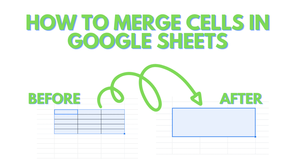
So first of all, let’s understand what merging cells mean. Merging cell refers to the combination of two or more cells to have one large cell.

It is commonly used in making the header rows but the point here is that merging can be in the form of Rows and Columns.

Whenever working on Google Sheets, you may come across the need to merge a few cells so that your table looks professional.

To do so, you just need to follow a few easy steps that you will learn in this tutorial and Boom! your task is done.

There are 2 methods how you can easily merge cells in Google Sheets:

1. By using the Format Tab option.
2. By using Merge Cells Button in the Ribbon.

How to Merge Cells In Google Sheets

To merge cells in Google Sheets use either of these two methods:

Method 1

1. Select the Cells
2. Click the Format Option
3. Go to the Merge Cells Command
4. Select Your Required Merge Type
5. Your Cells will be Merged

Method 2

1. Select the Cells
2. Click on the Merge Cells Button (OR Select Your Required Merge Type from the Dropdown)
3. Your Cells will be Merged

Merging Cells in Google Sheets Video Tutorial

How to Merge Cells In Google Sheets – Step-by-Step

Let’s just make an easy table and follow the necessary steps to merge the cells.

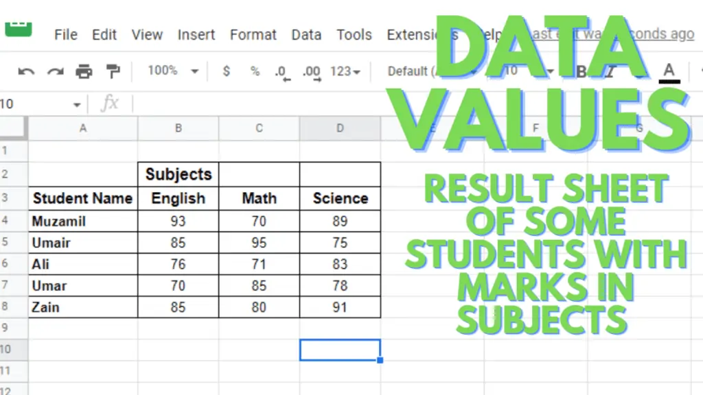
For example, a result sheet in which I have a list of a few students and their marks in the major subjects.

Now, as you can see the above data is well-formatted, have the heading bold, borders applied, everything nice…

RIGHT???

Of course, NOT.

Not everything is fine. Did You notice the issue???  I hope you did.

So, you found the problem in the above table that the Subjects heading should be somewhere in between the three columns of the three subjects.

Then, it will look better. Let’s now fix it by merging cells in Google Sheets.

Method 1 – Using the Format Tab Option to Merge Cells

Step 1 – Select the Cells

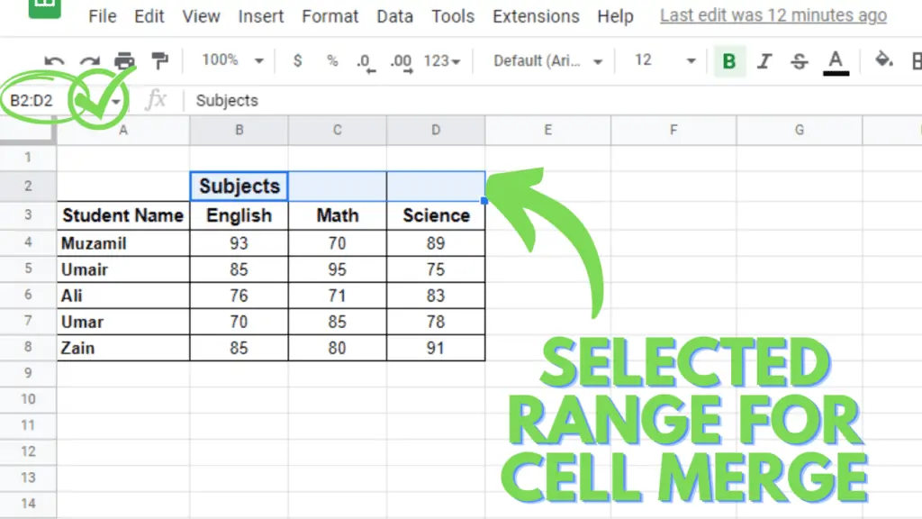
For merging the cells, first of all, we need to select all the cells that you want to merge so that they may make a good header for the table or fulfill any other purpose that you need to do.

In my case, I need to select the cells from B2:D2 (blue highlighted), so that the three cells will have the heading of Subjects in the center once we are done with merging.

Step 2 – Click the Format Option

After selecting the cells, you want to merge, the next step is to click on the Format Tab in the Toolbar (Ribbon).

You may find it just under the Title bar. As soon as you click on the format tab a list of commands will appear in front of you.

Step 3 – Click Merge Cells Command

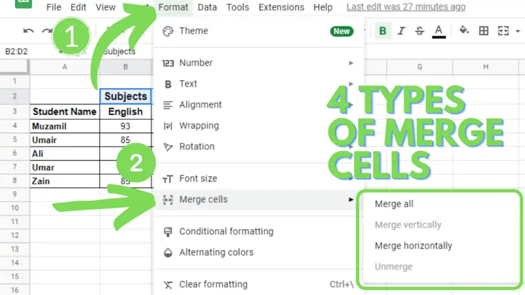
As a list of commands appears in front of you, the next step is to find the Merge cells command from among them and click on that.

As soon as you hover your mouse pointer or click on that Merge cells option, you will see 4 types of Merge cells that will appear in front of you:

1. Merge all
2. Merge vertically
3. Merge horizontally
4. Unmerge

4 Types of Merge Cells

Let me briefly introduce them so that you may not find it difficult to choose which type you should choose in your situation.

1. Merge All

The Merge All type is used when you need to make one large cell by merging cells vertically and horizontally both. This means that you are selecting cells from a row and a column at the same time and merging them all up to form one big cell.

2. Merge Vertically

Similarly, if you are merging cells of the same column then your choice will be Merge Vertically because it merges the cells vertically, and again you know that cells vertically arranged in the spreadsheet form the columns.

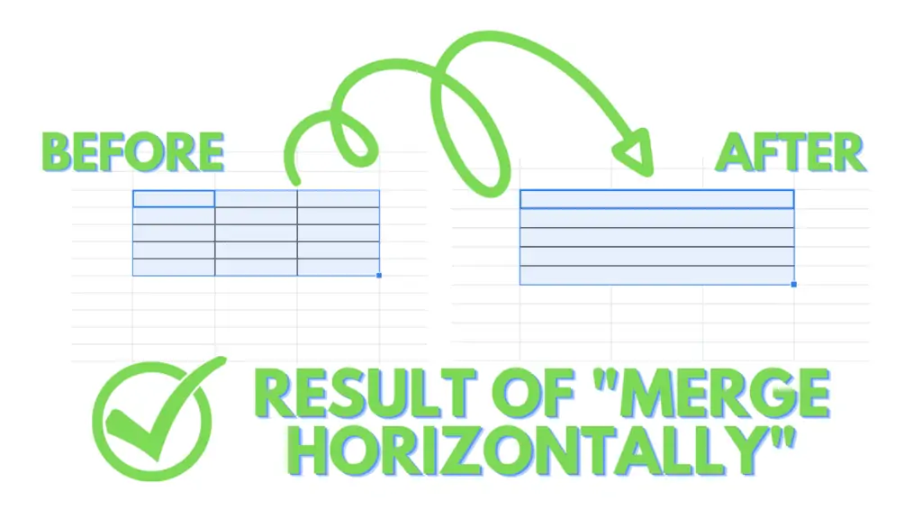
1. Merge Horizontally

If you are merging the cells of the same row then you will be selecting the Merge Horizontally type as it combines the cells horizontally which we know makes the rows of our spreadsheet.

(Note: All these merge types are not limited to applying on a single row or column. You can also select cells from two or more rows and columns and merge them too.)

1. Unmerge

The last is the Unmerge option. Despite like others, its function is not the same as all others. This command is the opposite of the merge command.

Just as you click on the unmerge option it will change your merged cell (that one large cell) into all the separate cells that you had selected for the merging process.

In my example, I will be selecting the Merge All OR Merge Horizontally type as I need to merge the cells in a row (horizontally).

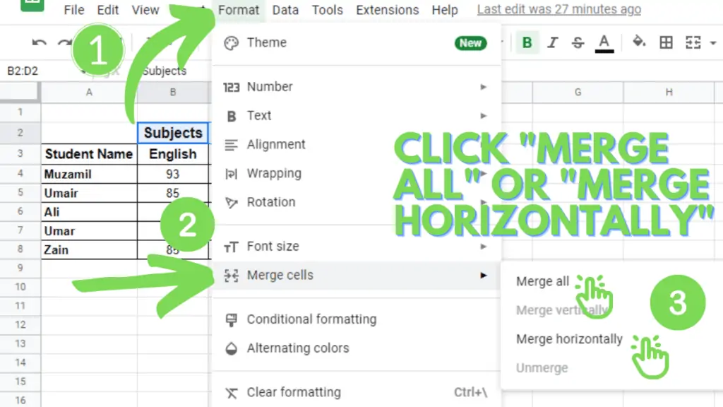
Note that the “Merge vertically” & “Unmerge” options are grayed out because I have selected the cells from one row only and yet unmerged.

When we select cells from two or more rows, the Merge vertically type will be active and when we select some already merged cell(s), the Unmerge option will be available for its application.

Step 4 – Your Cells will be Merged

You will notice that just as you select any of the Merge All OR Merge Horizontally types, all three cells have been merged together into a single larger cell.

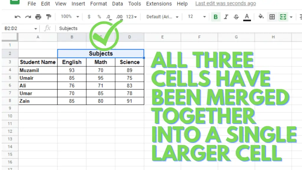
That’s how the Merge Cells Command works.

(Note: if you are worried that your text isn’t in the center then just made its alignment center from the alignment option in the Ribbon and your text will come where you want it to be)

Method 2 – Using Merge Cells Button in the Ribbon in Google Sheets

Step 1 – Select the Cells

The first step is the same for both methods. Again, you need to select all the cells you want to merge (vertically or horizontally).

I’m again going to repeat the same example so I will be again selecting cells B2:D2 for my example.

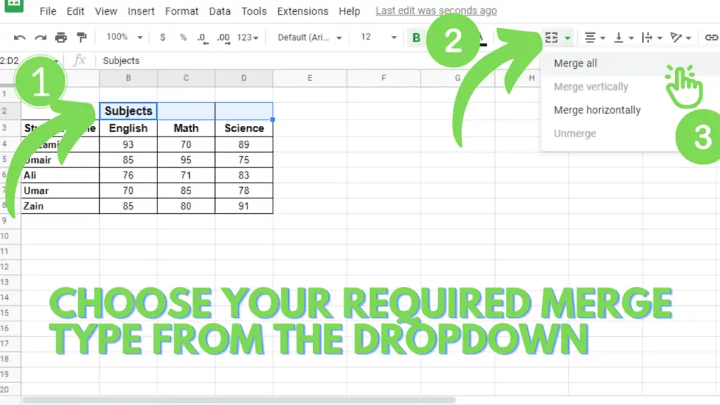
Step 2 – Click on the Merge Cells Button

So, in this method, you don’t need to go to the Format tab and then to merge cells command.

You also have an access to the merge cells command on the Ribbon in the Google Sheets.

It is called the Merge Cells Button/Icon. It does the same work as the Merge cells command in the Format Tab does.

Just as you select your cells and click on the merge icon your cells automatically get merged.

And let’s say that you need to have an access to the options of merge like merge horizontally or vertically then just click on the arrow (Dropdown) that you see next to the Merge icon.

It will give you all the options. Select your required merge type and click on it. Your selected cells will be merged.

Step 3 – Your Cells will be Merged

The results are the same. You again get the selected cells merged as per your requirements.

Conclusion on How to Merge Cells In Google Sheets

There are two ways to merge cells in Google Sheets. You can either use the Format Tab option or merge cells by using the Merge Cells button in the ribbon.

These were two easy methods by which you can merge cells in Google Sheets. I hope this tutorial was helpful to you.