How to Highlight Duplicates in Google Sheets – 4 Quick Steps

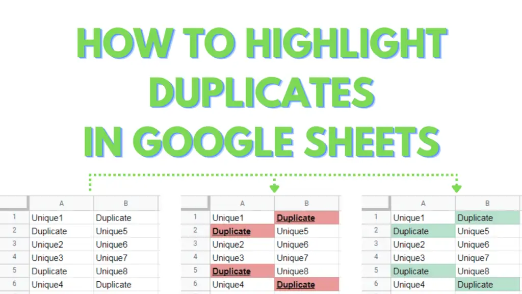
In this tutorial, I will show you how to highlight duplicates in Google Sheets using conditional formatting.

Conditional formatting allows you to set criteria that Google Sheets will use to whether or not to apply a custom format, to ideally highlight duplicate entries within a range.

I will discuss how to set up conditional formatting to highlight duplicates within a row, within a column, or within an array of rows and columns.

Next, I will discuss what formatting style we can apply to a duplicate entry to highlight it.

How to Highlight Duplicates in Google Sheets

To Highlight Duplicates in Google Sheets, follow these steps:

1. Select a Column, Row, or Range to scan for Duplicates
2. Click on Format Menu, then click on Conditional Formatting
3. In the Conditional format rules panel, in the “Format cells if…” dropdown selection, select “Custom formula is”
   1. If the selection is a range with a single-column dimension, use the formula:
      “=IF(COUNTIF([Absolute Range],[Top Row Address])>1,TRUE,FALSE)”
   2. If the selection is a range with a single row dimension, use the formula:
      “=IF(COUNTIF([Absolute Range],[First Column Address])>1,TRUE,FALSE)”
   3. If the selection is range with multiple rows and columns, use the formula:
      “=IF(COUNTIF(FLATTEN([Absolute Range]),[First Column & Row Address])>1,TRUE,FALSE)”
   4. In the Conditional format rules panel, set up how to highlight duplicates under the Formatting style section

For this tutorial, I will provide a sample file that will have 3 sheets.

One sheet will have data along a single row, the other would have data in a single column, and the last will have data across multiple rows and columns.

The data in these sheets will be a lot and some of them will be duplicates.

Simply make a copy by accessing the file through this link, then click on the file under the menu bar, then click on make a copy.

A dialog box should appear.

Within it, you can provide a filename for the copy then click “Make a Copy”.

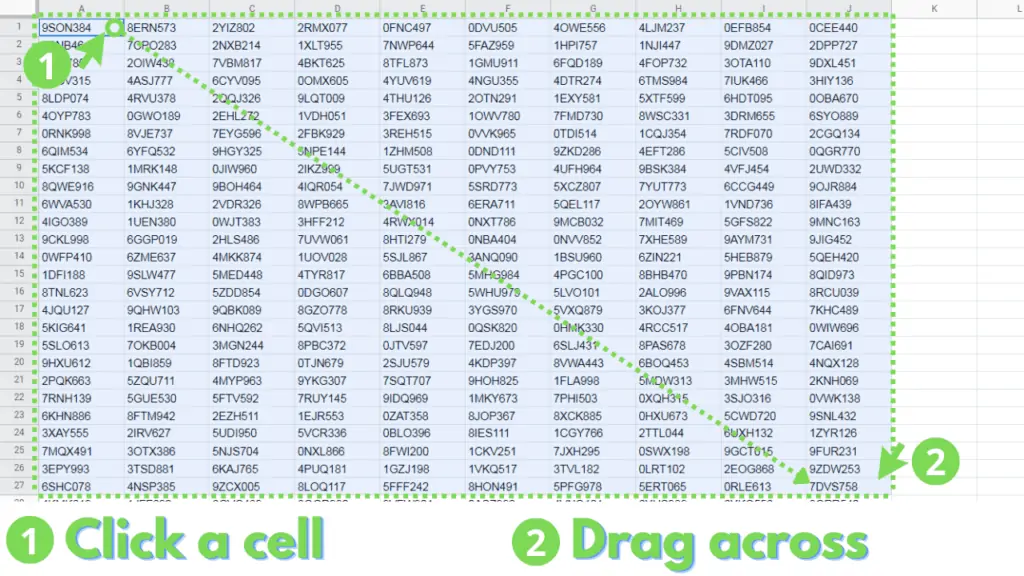
Step 1 – Select a Column, Row, or Range to scan for Duplicates in Google Sheets

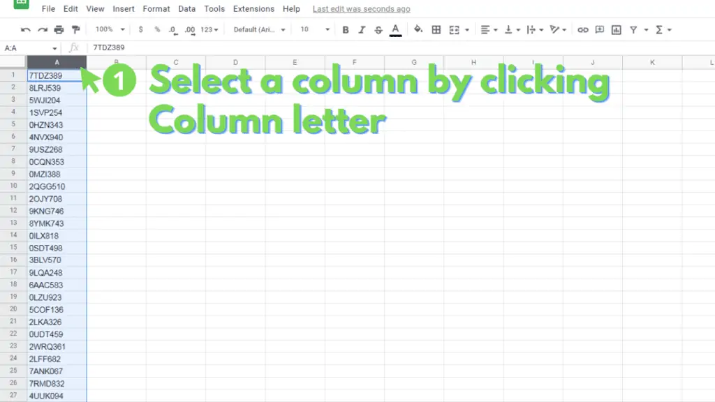
You first need to highlight the range that you want to find duplets in. If the range is a column, simply select the Column Letter from the top of the worksheet, by clicking on it.

If the range is within a column, drag and select from the topmost cell downwards.

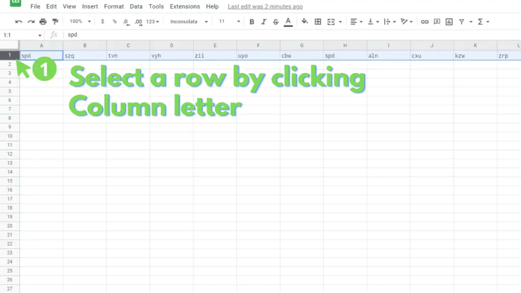
If the range is a row, simply select the row number from the left of the worksheet by clicking on it.

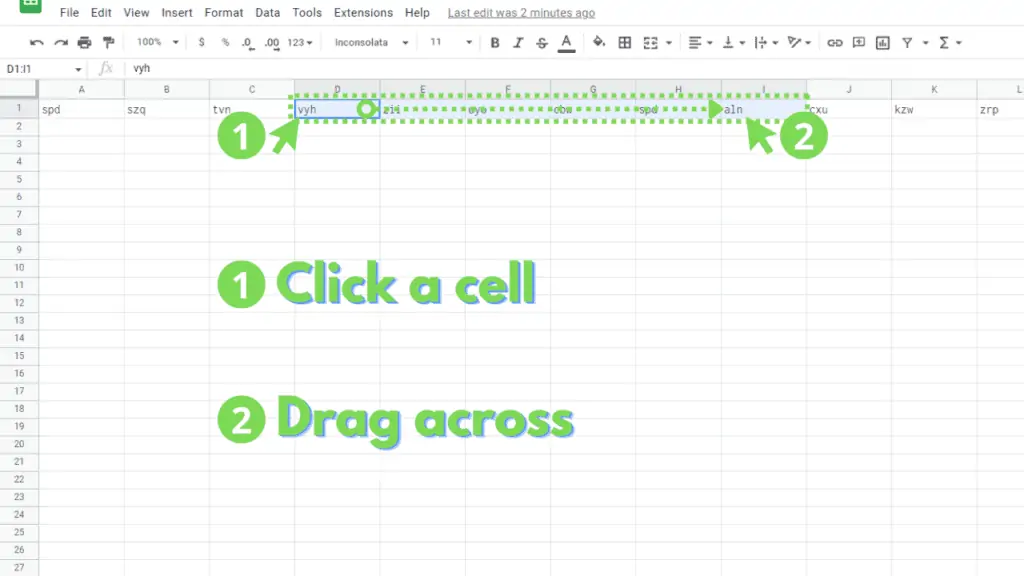
If the range is within a row, drag and select from the leftmost cell to the right.

If the range is an array composed of multiple rows or columns, select the cell from the top-left corner then drag toward the lower-right corner of your selection.

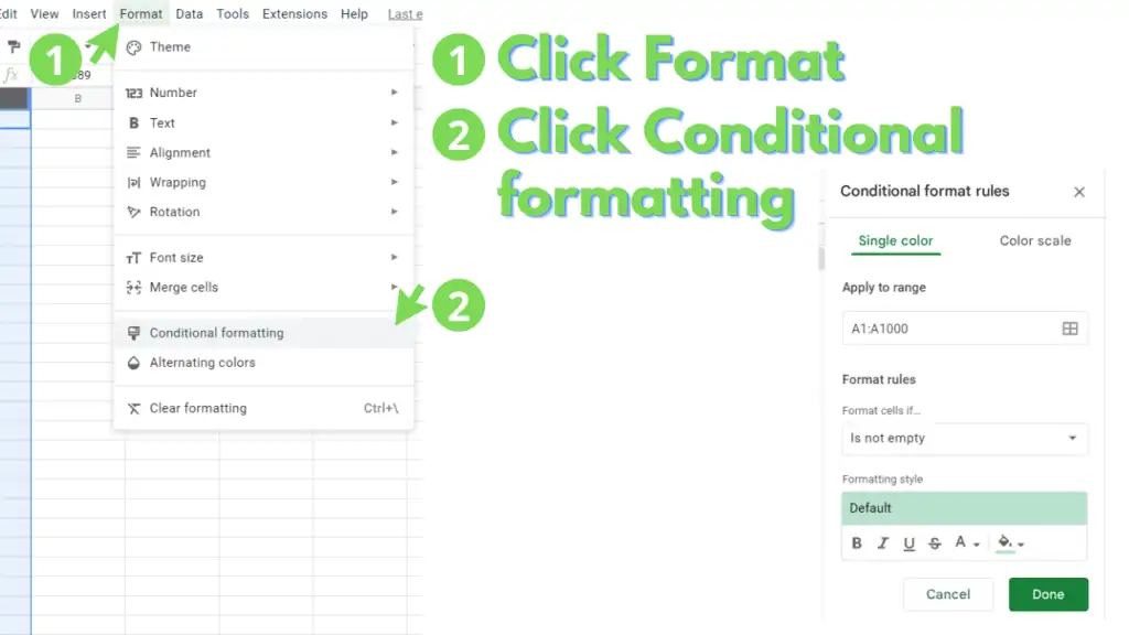
Step 2 – Apply Conditional Formatting on the Selection

Now that you’ve selected a range to scan for duplicates, we will need to apply conditional formatting on the range, in preparation for the formula and formatting that we will use.

To do this, simply click on “Format” from the “Menu Bar”, then select “Conditional Formatting”.

This should bring up the “Conditional format rules” panel:

Step 3 – Apply a Custom Formula to identify Duplicate Entries from the Selection

Conditional formatting works through the use of logic.

Basically, you set up a rule, or several rules, then if the conditions are met or return a result of TRUE, then the formatting applies.

The default conditional formatting highlights a cell that is NOT empty:

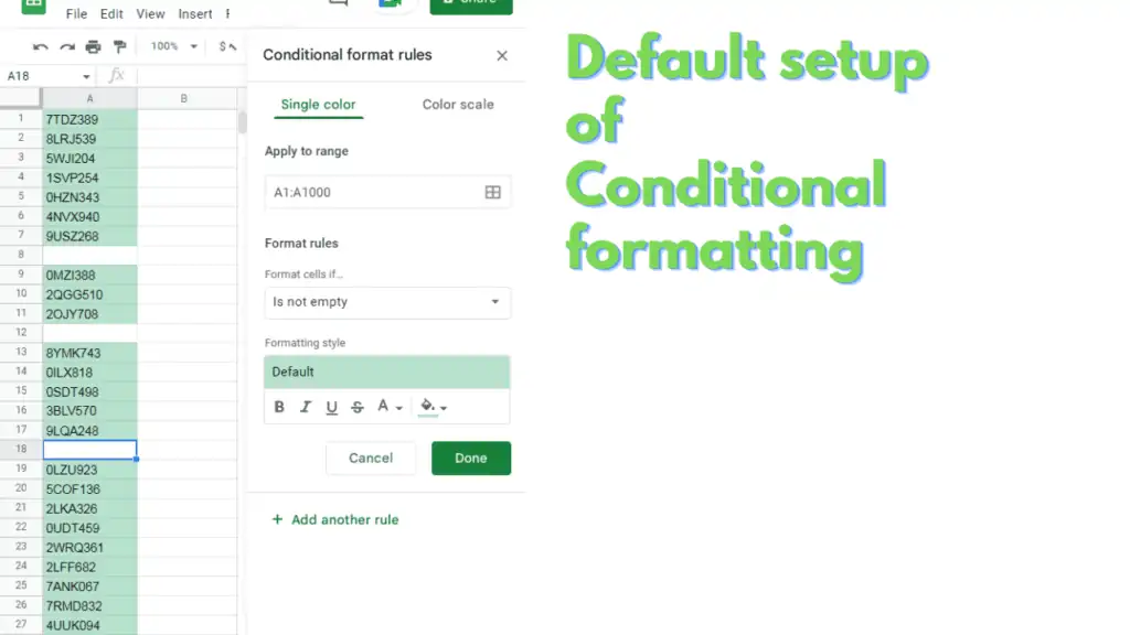
Any FALSE result through the conditions that were set up would exclude the cell from the Conditional Formatting, defaulting to whatever formatting was set up for the cell.

Let’s now move on to the use of custom formulas to set up more advanced criteria to apply formatting to a selection.

To toggle the use of custom formulas in the “Conditional format rules” panel, click on the drop-down selection under “Format cells if…” and select “Custom formula is”.

This should open up a new field with a default label of “Value or Formula”, where you will enter one of the formulas we will discuss.

To identify duplicate entries in a column in Google Sheets, modify this formula by replacing [Absolute Range] with the absolute form of the range of your selection, and by replacing [Top Row Address] with the address of the topmost cell in your selection:

=IF(COUNTIF([Absolute Range],[Top Row Address])>1,TRUE,FALSE)

As an example, to Identify duplicate entries in the range A5 to A20, the formula should be as follows:

=IF(COUNTIF($A$5:$A$20,A5)>1,TRUE,FALSE)

To identify Duplicate Entries in a Row, modify this formula by replacing [Absolute Range] with the absolute form of the range of your selection, and by replacing [First Column Address] with the address of the leftmost cell in your selection:

=IF(COUNTIF([Absolute Range],[First Column Address])>1,TRUE,FALSE)

As an example, to Identify Duplicate Entries in the range C1 to N1, the formula should be as follows:

=IF(COUNTIF($C$1:$N$1,C1)>1,TRUE,FALSE)

To identify duplicate entries in a range with multiple rows or columns, modify this formula by replacing [Absolute Range] with the absolute form of the range of your selection, and by replacing [First Column & Row Address] with the address of the cell in the top-left corner of your selection:

=IF(COUNTIF(FLATTEN([Absolute Range]),[First Column & Row Address])>1,TRUE,FALSE)

As an example, to identify duplicate entries in the range B2 to H20, the formula should be as follows:

=IF(COUNTIF(FLATTEN($B$2:$H$20),B2)>1,TRUE,FALSE)

Step 4 – Apply Formatting style to Highlight Duplicate Entries

Once you have modified and entered the formulas we discussed, we can now move on to selecting formatting styles to highlight duplicate entries in our selection.

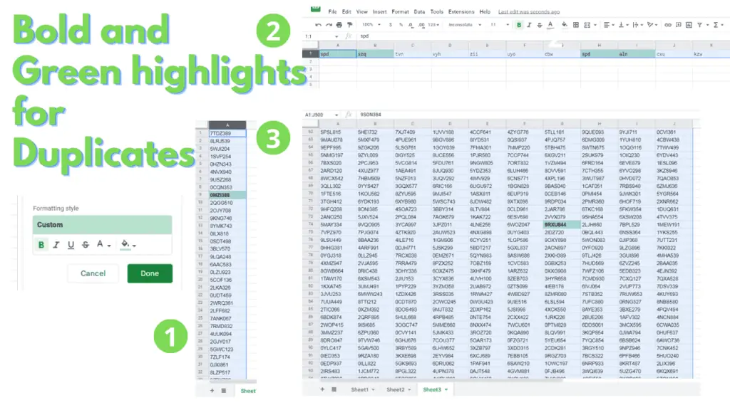
To do this, simply move over to the “Formatting style” section of the “Conditional format rules” panel and toggle or customize the format.

To have the duplicates appear in bold font while highlighted by a light-green color, the formatting style should be set up like the following:

You now know how to highlight duplicates in Google Sheets.

Expand on how to highlight duplicates in Google Sheets by reading the article how to copy conditional formatting.

Conclusion on How to Highlight Duplicates in Google Sheets:

To highlight duplicates in Google Sheets select a range to scan for duplicates. To select a single column, click on the Column Letter from the top. To select a single row, click on the Row Number from the left.

To select from a single row across multiple columns, click and drag from the first column to the rightmost column of the same row. To select from a single column along multiple rows, click and drag from the first row to the last row of the same column.

To select a range with multiple rows or columns, click and drag from the top-left corner of what you would like to select to the bottom-right corner.

Next, apply Conditional Formatting to your selection by clicking on Format from the Menu Bar, and by clicking on Conditional Formatting.

Following that, set up the use of a Custom Formula by selecting “Custom formula is” from the drop-down selection directly under the “Format cells if…” label.

If you’re trying to Highlight Duplicates from a selection within a single row or a single column, modify the following formula by replacing [Absolute Range] with the absolute form of your selected range, and by replacing [Top Row Address] with the cell address on the topmost or leftmost cell of your selection:
=IF(COUNTIF([Absolute Range],[Top Row Address])>1,TRUE,FALSE)

When trying to Highlight Duplicates from a selection with multiple rows and columns, modify the following formula by replacing [Absolute Range with the absolute form of your selected range, and by replacing [First Column & Row Address] with the cell address on the top-left corner of your selection:
=IF(COUNTIF(FLATTEN([Absolute Range]),[First Column & Row Address])>1,TRUE,FALSE)

Finally, set up what formatting you want to use to Highlight Duplicates using the options supplied under the “Formatting styles” section of the “Conditional format rules” panel.