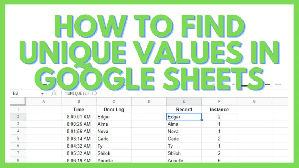
In this tutorial, I will show you how to find unique values in Google Sheets.
Finding a word or value in a spreadsheet with thousands of rows can be a nightmare but is doable with different find features and functions. But identifying the unique values in thousands of rows gets really difficult this way.
How to Find Unique Values in Google Sheets
- Identify the range where you want to find unique values in
- Select a cell in a clear column
- Type in =UNIQUE(range)
- Hit enter or click another cell
Find Unique Values in Google Sheets Video Tutorial
2 Ways to Find Unique Values in Google Sheets
I’ve been using different ways to find unique values in Google Sheets over the year as it is useful in a number of situations. You can use it for records computations, and even financial spreadsheets.
Below I have listed two easy ways how to find unique values:
1. Using the Remove Duplicates Menu Option in Google Sheets
The first method is done by using the menu option.
Before starting, you must have your range selected.
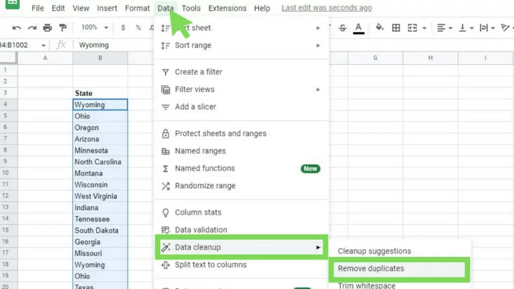
Then, go to ‘Data’. And then to ‘Data cleanup. Lastly, select ‘Remove duplicates’.
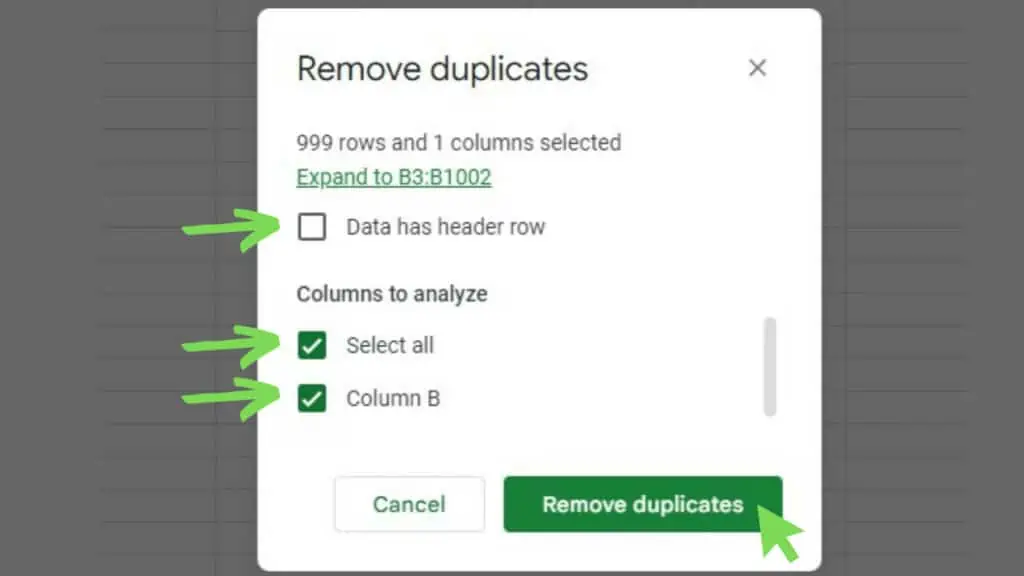
This will bring up the ‘Remove duplicates’ window with some options that you can select depending on your requirements.
First is the ‘Data has header row’. If you have selected a range including a header or a title at the top, tick this checkbox.
Next is the ‘Columns to analyze’. If you selected a range with more than one column, each one will show up here giving you the option to select which ones are going to be cleaned up.
Once you’re satisfied with your settings, hit ‘Remove duplicates’.
You’ll see a confirmation window indicating how many duplicate rows were found and then removed – as well as the number of unique rows that remain.
Hit ‘OK’ to proceed.

You will then see that the row that you’ve selected would be shorter depending on how many rows were removed during the cleanup.
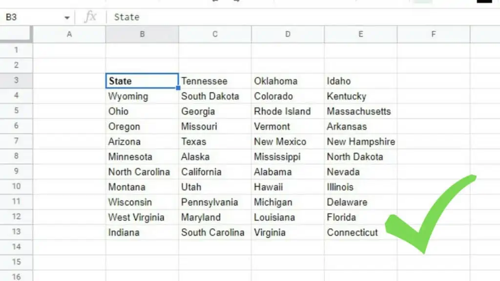
I’ve rearranged the results below to 4 columns so you can see all 43 remaining values (except the header).
This is useful if you have a static list that you want to clean up and you no longer need to keep the original data.
For other purposes, I recommend you use the UNIQUE Function to find unique values in Google Sheets.
2. Using the UNIQUE Function
Another way to find unique values in Google Sheets is via the UNIQUE Function.
The basic syntax of the UNIQUE Function is
=UNIQUE(range)
Where range is the data you wish to filter for unique values.
In the example below, I have a list of 23 companies. On a separate cell (D4), I then used the UNIQUE Function on this existing range.
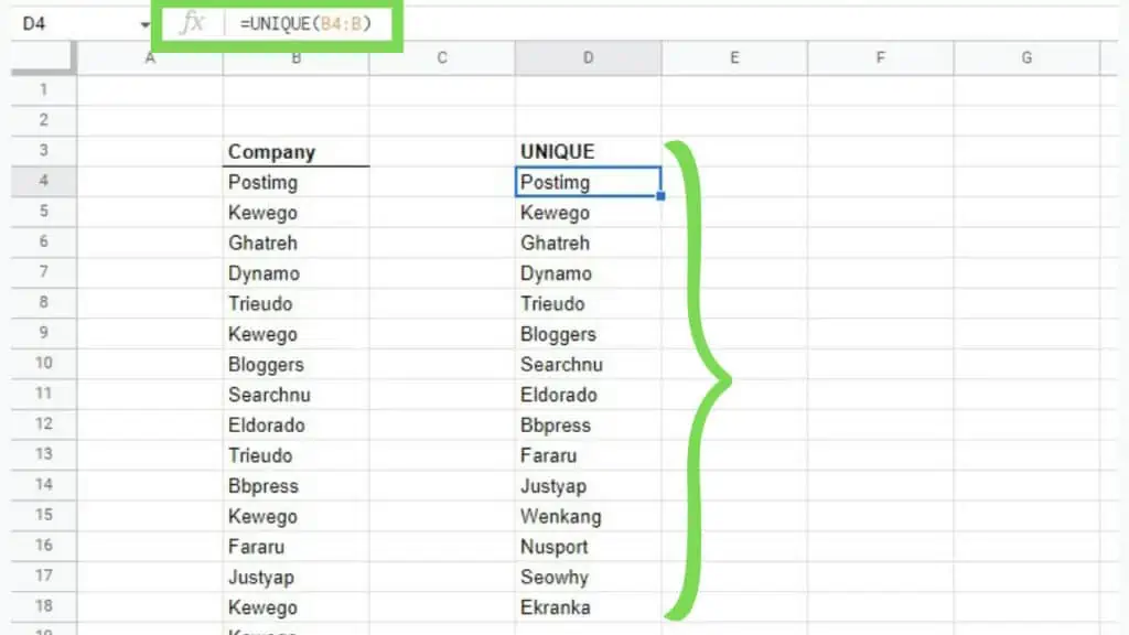
In doing so, I got a shorter list of 15 unique companies.
Other than the range parameter, UNIQUE actually has 2 more optional parameters.
The full syntax of UNIQUE is
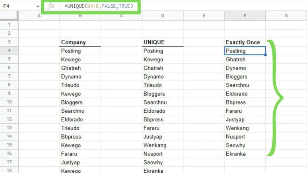
=UNIQUE(range, [by_column], [exactly_once])
Both of the added parameters are optional and accept either TRUE or FALSE values where both are FALSE by default.
[by_column] is set as TRUE only if you want the filtering to be done horizontally while [exactly_once] is set as TRUE only if you want to exclude values that appear more than once in your selected range.
In the example below, I’ve set the [exactly_once] parameter as TRUE causing ‘Kewego’ and ‘Trieudo’ to not be included since they appear multiple times in the selected range.
This is how you use UNIQUE to find unique values in Google Sheets.
2 Ways to Use UNIQUE With Other Functions
I often recommend using UNIQUE over the menu option to find unique values in Google Sheets as it is more versatile and is usable with other functions giving you the ability to use it for more complex situations.
Below are two examples where I use the results of UNIQUE in tandem with other functions.
1. Using COUNTIF with the UNIQUE Function
One of the best partners of UNIQUE is the COUNTIF Function. Combining these two allows you to find unique values in Google Sheets and count each time the unique value appeared in the selected range.
In the example below, I have a small dataset of student names and each one’s favorite color. I used the UNIQUE Function on the set of colors to know what are the unique colors for this example.
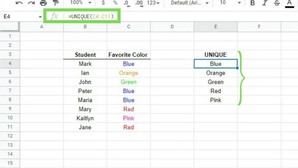
Now, I know that there are five unique colors that are the students’ favorites but I do not know how many students like each color.
To define this information, I just need to use COUNTIF on the results of the UNIQUE Function.
The syntax of COUNTIF is
=COUNTIF(range, criterion)
In this example, we assign the range as the original dataset while the criterion will be for each result of the UNIQUE Function.
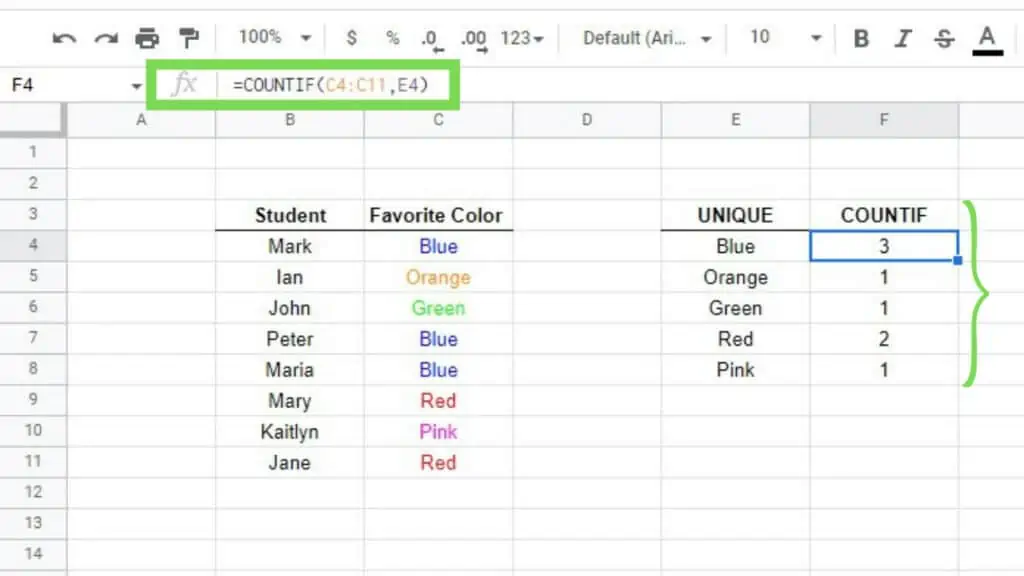
Now I know that there are three students who like ‘blue’, two students who like ‘Red’, and a single student each for the rest of the colors.
This is extremely useful for order or inventory records where you can apply the UNIQUE Function on the products and use COUNTIF on UNIQUE’s output to know how much of each product you have on an order or inventory.
2. Using FILTER and LEN with the UNIQUE Function
This is another useful way to use the UNIQUE Function, this time with FILTER and LEN.
Using this method, we’ll be able to find the unique values in Google Sheets where there are multiple columns in the range that we wish to filter.
The thing is, you can only use UNIQUE one column at a time and that means that you won’t be able to filter out duplicate values that are in one column and in another.
That is where the FILTER and LEN Functions come in.
The syntax for FILTER is
=FILTER(range, condition1, [condition2, …])
While for LEN it’s
=LEN(text)
And we’ll use a compound function of these two where LEN will be the condition value for FILTER.
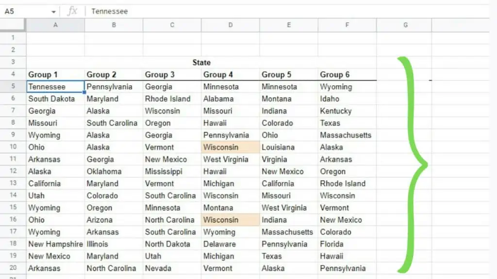
The example dataset below consists of 6 columns with 16 values each.
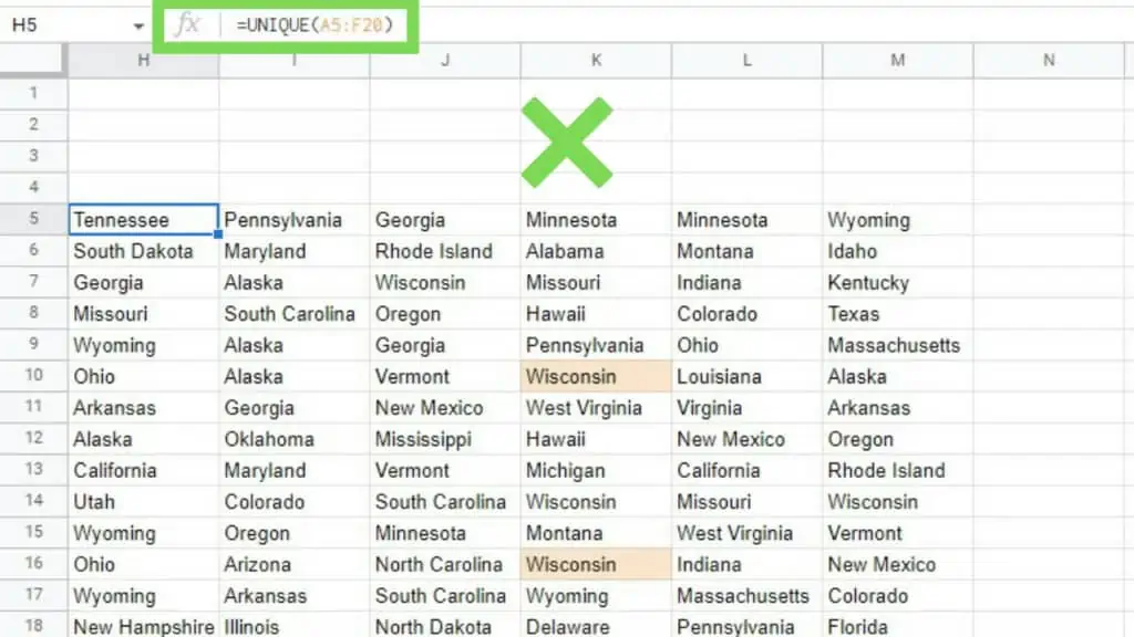
If I use the UNIQUE Function as it is, you can see that nothing actually happened. It just copied the entire range.
To make this work, we’ll use the aforementioned compound function of FILTER and LEN.
The syntax is:
=FILTER({range1;range2;…}, LEN({range1;range2;…}))
Where each individual column will be one range followed by another, separated by a semi-colon all enclosed by a pair of brackets.
Take note that the contents of the range parameter of FILTER are exactly the same as the text parameter of LEN.
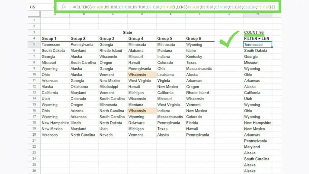
This will put everything into a single column. The entire result can now be used as the range for our UNIQUE Function. Meaning, we can use it by making it the parameter for UNIQUE as seen below.
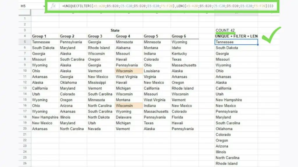
I’ve added a COUNTA Function on cell H3 to display the difference of the total number of values in the range H5:H.
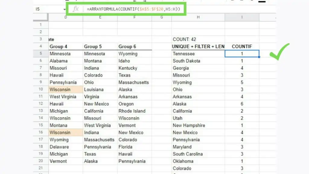
Similar to the previous method, once I got the results of UNIQUE, I can then use it for COUNTIF letting me know the number of times a state was mentioned in my original dataset.
Using different functions with UNIQUE will help you do various things after you find unique values in Google Sheets.
There are also other applications of find in Google Sheets such as the Find and Replace feature.
Frequently Asked Questions about How to Find Unique Values in Google Sheets
Why am I getting a #REF! error when I use UNIQUE to find unique values in Google Sheets?
To avoid getting a #REF! error when you use UNIQUE to find unique values in Google Sheets, make sure that you have enough empty cells below the cell where you input your formula to accommodate the output of UNIQUE. You can find the cell to fix in the error message.
Can I use a range with numerical data to find unique values in Google Sheets?
You can use numerical data as the range for UNIQUE in Google Sheets but take note of some conventions such as percentage where 0.01 is the same as 1% so only the first of these values will be kept as part of UNIQUE’s output.
Conclusion on How to Find Unique Values in Google Sheets
To find unique values in Google Sheets by first identifying a range where you want to find unique values and then selecting a cell in a clear column or with enough space below it to accommodate the results of the UNIQUE Function. Next, type in the formula: “=UNIQUE(range)”. Lastly, hit enter or click another cell.

