How to do a Checkmark in Google Sheets – 4 Easy Steps

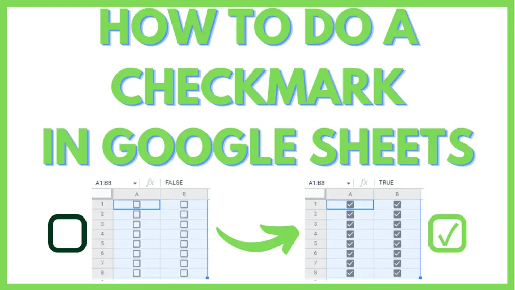
In this tutorial, I will show you how to do a checkmark in Google Sheets.

Google Sheets, being a spreadsheet application, is ideal for storing lists along rows or columns.

A good way to track the status or progress of these items is through the use of checkmarks.

Checkmarks are locally defined as checkboxes, a data validation option in Google Sheets.

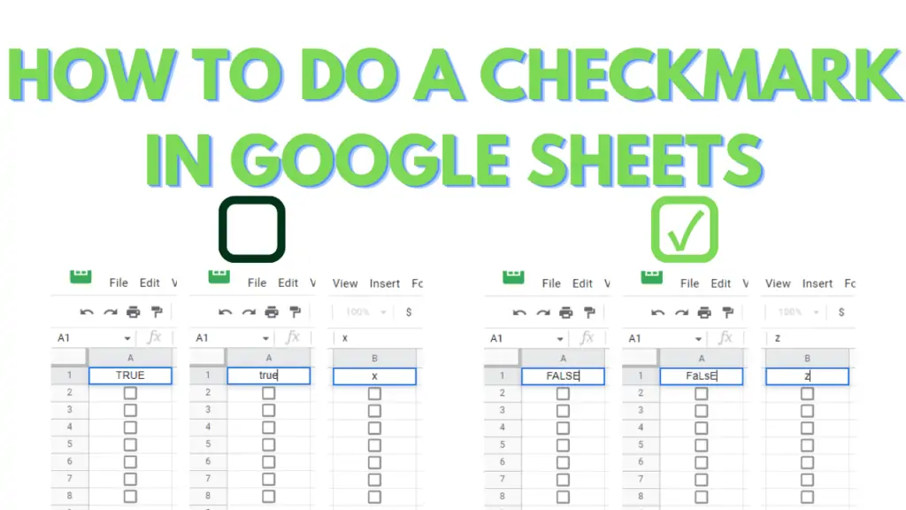
They store boolean values, such as the default TRUE or FALSE, or any other boolean pair that you want to use, like Yes or No, Up or Down, etc.

State	Default	Boolean 1	Boolean 2	Boolean 3
Checked	TRUE	x	Yes	Up
Unchecked	FALSE	z	No	Down

While visually, a checkbox will show a ticked (checked) or unticked (unchecked) box, internally, they will store the boolean pair that you choose.

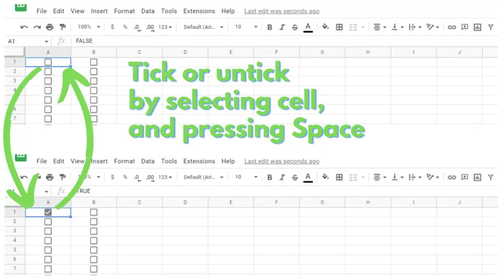
Additionally, you can toggle a checkbox from a ticked state to an unticked one and vice versa by selecting it and pressing the spacebar.

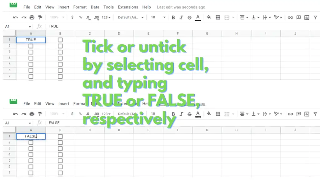
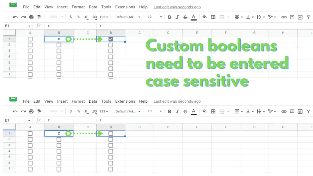
It is also possible to toggle the state of a checkbox by typing either of the boolean values that you chose.

Typing “x” in a checkbox that is set to have “x” or “z” as its boolean values will tick it, while typing “z” will untick it.

Checkboxes, together with Conditional Formatting that you can copy to other ranges, are effective visual cues for easier viewing of your Google Sheets files.

How to do a Checkmark in Google Sheets

To do a Checkmark in Google Sheets, follow these steps:

1. Select a Range that you will turn into Checkboxes
2. Click Data Menu, then select Data Validation
3. Select Checkbox in the Criteria Dropdown
   1. Keep the use Custom Cell Values checkbox unticked and click Save
   2. Tick the use Custom Cell Values checkbox, fill in the Boolean Values, and click Save
4. Tick or untick a single Checkbox by selecting it and pressing space
   1. Tick a range by selecting a range and pressing space
   2. Untick a range by selecting a range, and pressing space twice

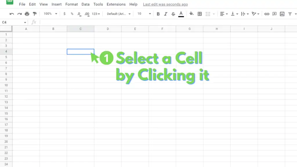
Step 1 – Select a Range

A checkmark, or checkbox, is a data validation option that has to be applied to cells in Google Sheets, whether individually or as a range.

There are several methods you can use to select a range, the first of which is simply to simply select a cell by clicking it.

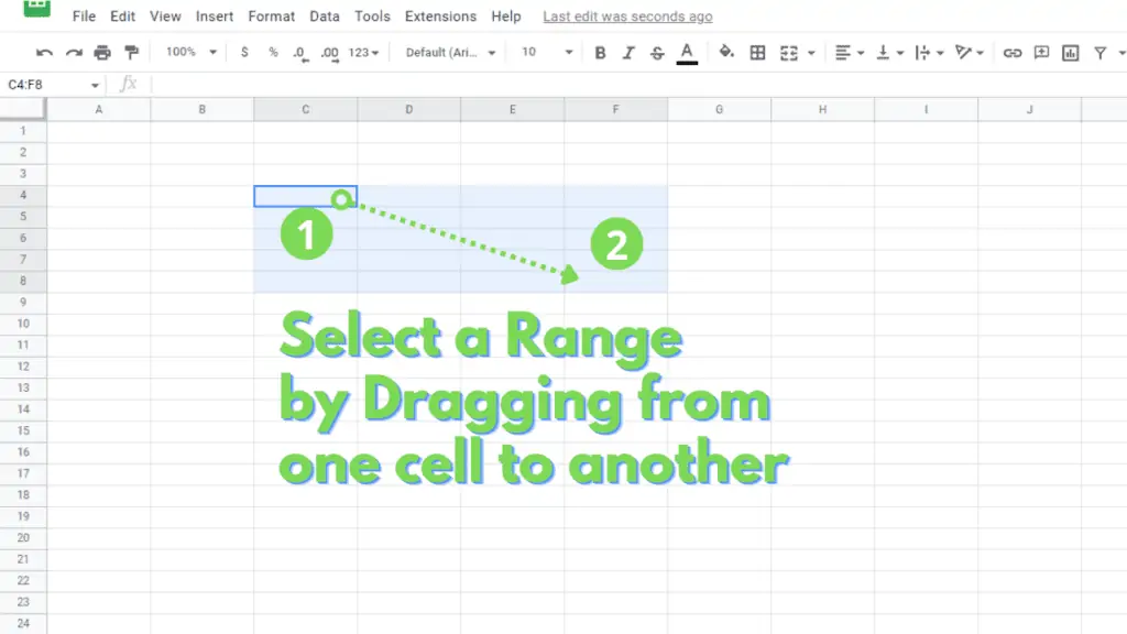
Another is to select a range, which itself can be divided further into different methods.
One such method is selecting a range by dragging from a selected cell.

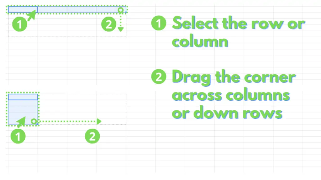
Another method is selecting additional row(s) or column(s) from selected row(s) or column(s) in Google Sheets.

This method ensures that the final selection will match the dimensions of your initial selection of row(s) or column(s).

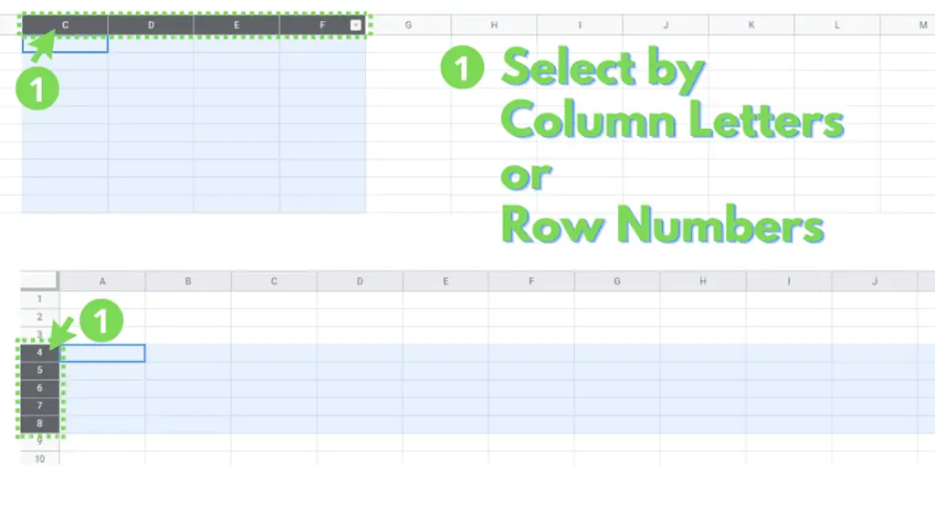
The next one is by selecting a whole row or column through their column letter(s) or row number(s).

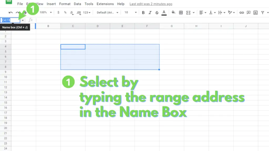
The final method is to enter the cell or range address in the name box.

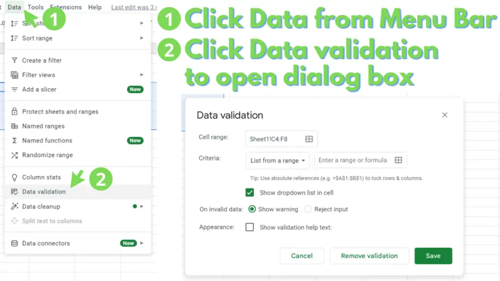
Step 2 – Enter Data Validation Menu

Now that you’ve selected a cell or range, the next step is to convert the selection into a checkbox to tick or untick later.

To do that, click data under the menu bar, then click data validation. Doing so should open up a different dialog box.

Step 3 – Setup Checkbox as Data Validation

Inside the data validation dialog box, click the dropdown selection beside the criteria section and select checkbox to show the checkbox options in the dialog box:

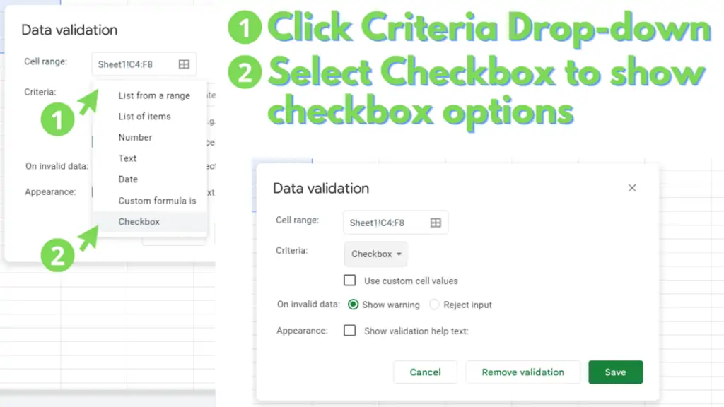
You can go ahead and click save if you choose to use the default boolean pair TRUE or FALSE.

If you want to use a different boolean pair as the internal values for a ticked or unticked checkbox, check the “Use custom cell values” checkbox.

Once checked, a pair of new textboxes will appear:

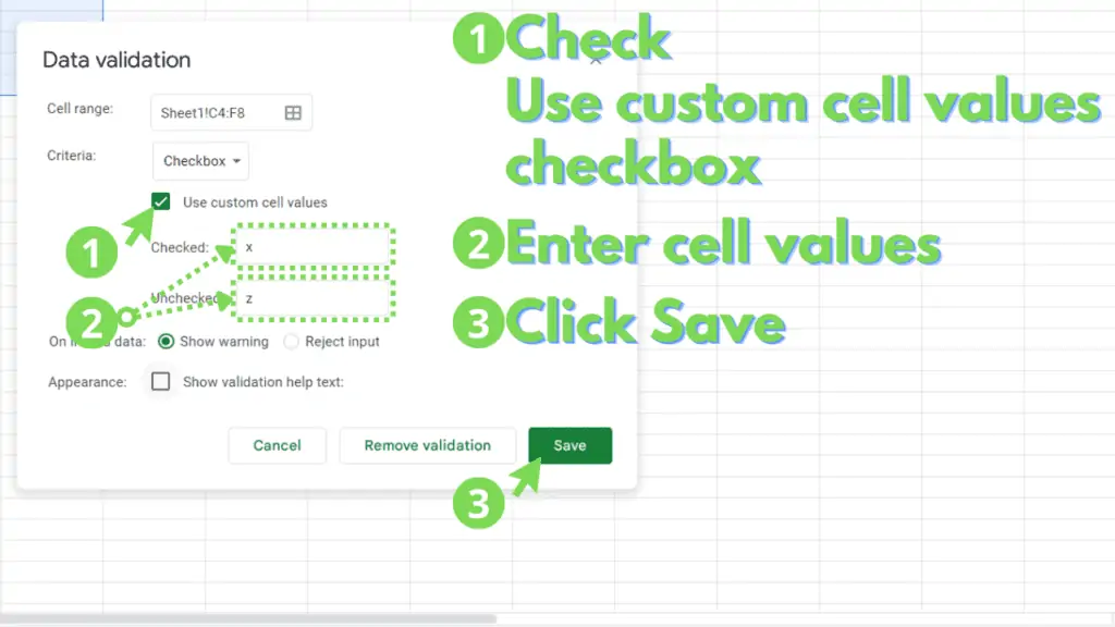
Fill these in with your choice of a boolean pair, then click save.

Step 4 – Tick or Untick a Checkbox or Checkboxes

Now that you’ve turned a cell or a range into checkboxes, you can go ahead and tick or untick them.

There are several ways to do it, and some are more efficient than others.

To tick or untick an individual checkbox, simply select it, then press space.

You can also type in the boolean value itself to tick or untick the checkbox.

However, when typing in the boolean value, remember that if the checkbox is not set up to “Use custom cell values”, you can enter TRUE or FALSE in a non-case-sensitive manner.

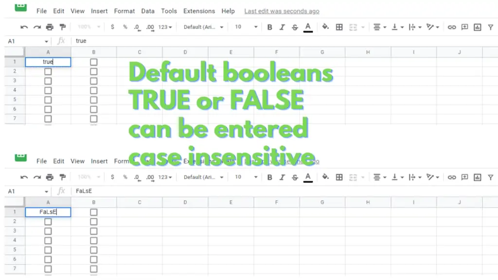
Otherwise, what you type in has to match the case of your chosen boolean pair.

It is possible to mass-tick checkboxes by selecting them and pressing space.

If there is a ticked checkbox in the selection it will remain ticked rather than unticked.

Finally, to mass untick checkboxes, select the range, then press the spacebar twice.

The first spacebar ticks the whole selection, then the second press of the spacebar unticks the whole selection.

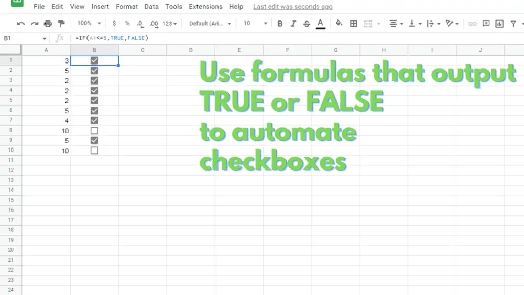
Also, since internally, checkboxes store a boolean value depending on whether it’s ticked or unticked, (TRUE or FALSE, Yes or No, etc.) you can also create formulas that output these boolean values.

A basic application is shown below, where a checkbox will be ticked if the number to its left is less than or equal to 5.

Now you know how to do a Checkmark in Google Sheets.

Frequently Asked Questions on How to do a Checkmark in Google Sheets

Conclusion on How to do a Checkmark in Google Sheets

To do a checkmark in Google Sheets select a cell or range that you want to turn into a Checkbox. Then click on Data from the Menu Bar, and click on Data Validation to open the Data Validation Dialog Box.

Next, in the Criteria Dropdown selection, select Checkbox. From here, you can use the default TRUE or FALSE values. You can also use custom Boolean Pairs by checking the “Use custom cell values” option, then supplying the ticked and unticked cell values that you want the cells to store. After choosing, click on the Save button.

Finally, you can tick or untick a cell by selecting it then pressing the spacebar, or by typing the custom cell values. When ticking or unticking a range, select the range first, then press space once to tick the range. When the selection is ticked, you can press spacebar again to untick.