The QUERY function in Google Sheets is extremely useful to present data.
The PIVOT function itself is most useful when you have multiple dimensions of data at hand.
In this tutorial, I assume that you already have some understanding of how the Google Sheets QUERY function works.
How to Create a Pivot Query in Google Sheets
To create a pivot query in Google Sheets use the QUERY function with the PIVOT function as one of its query parameters.
Example: =QUERY(A1:D51, “SELECT C, SUM(D) GROUP BY C PIVOT B”,1)
How to Create a Pivot Query in Google Sheets – Step By Step
To create a pivot query in Google Sheets, we’re going to be using the QUERY function with PIVOT as one of its ‘query’ parameters.
As an example, we can use the QUERY formula below:
=QUERY(A1:D51, “SELECT C, SUM(D) GROUP BY C PIVOT B”,1)
The PIVOT clause of the QUERY function is a bit tricky and requires some time and experience before you master it.
Basics of the QUERY Function in Google Sheets
Before proceeding to how the pivot query in Google Sheets works, it’s best to have a look at the basic syntax.
The basic syntax of the QUERY function is as follows:
QUERY(data, query, [headers])
The data parameter is for the actual range in your spreadsheet where the data you want to be processed is in.
The headers parameter is optional indicating if you want Google Sheets to recognize your dataset as having header rows, and if so, how many.
The focus in this section of this tutorial is the QUERY parameter.
This is where you’ll see complex lines such as:
“SELECT A, count(C), min(B), max(B), avg(B) GROUP BY A ORDER BY avg(B) DESC LIMIT 3”
Here are the basic keywords used for the QUERY parameter.
- select
- where
- group by
- order by
- limit
- label
These are non-case-sensitive so you may use them in an upper-case format as well. It’s also important to note that in using these keywords, they must be in order from left to right.
Using the PIVOT clause of the QUERY function in Google Sheets
Utilized in transforming specific values in columns into new columns, a pivot by a column ‘period’ would produce a table with a column for each distinct period that is displayed in the original table.
‘Pivot’ can be really useful when, for example, a chart containing lines to visualize illustrates each column separately as lines.
If you wish to make a separate line for each period, and ‘period’ is one of the columns of the source dataset, then a good way to do it would be to use a pivot query in Google Sheets to do the necessary data processing.
Take note that as a number of rows may have similar values for the pivot columns, pivot implies aggregation.
Also take note that when you use ‘pivot’ without using ‘group by’, the result table will contain exactly one row.
Pivot Query in Google Sheets Example – Sales Report Data
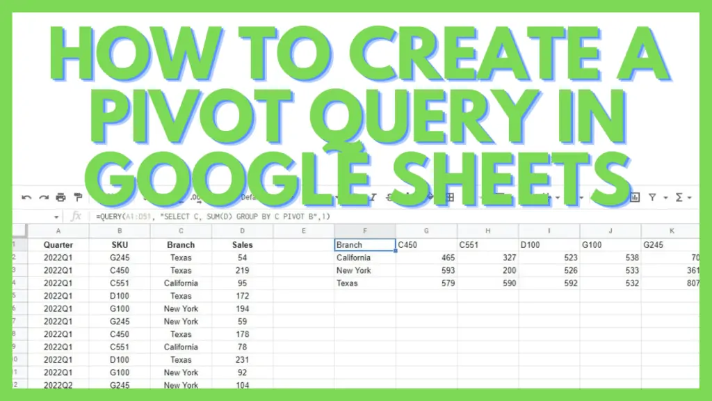
In the sample dataset below, we have five product SKUs: G245, C450, C551, D100, and G100. This is a sales report with sales for each SKU unit by branch location.

Let’s say we need to get the number of sales, by branch. To do that, we’ll use the following formula below:
=QUERY(A1:D51, “SELECT C, SUM(D) GROUP BY C PIVOT B”,1)
The query means
SELECT branch, SUM(sales) GROUP BY branch PIVOT by SKU
And the result will produce the following:

The PIVOT clause results in the SKUs becoming column headers. Afterward, the SUM and GROUP BY clauses calculate the values required.
At the start, we had four dimensions to the data we had which are: quarter, SKU, branch, and sales.
Using the aggregate functions and the pivot we moved the data to 3 dimensions: state, product, and units sold
Example QUERY function in Google Sheets: Payout Record Data Sample
This time, with the sample dataset below, we have five agents with IDs:100121, 105398, 105622, 115320, and 124008.
This is a payout record for agents given out on different dates.

With this one, what we need to get is the payout record, per employee, per day. To do that, we’ll use the following formula below:
=QUERY(A1:C51,”SELECT A,SUM(C) GROUP BY A PIVOT B”,1)
The query means
SELECT Date Filed, SUM(Payout) GROUP BY Date Filed PIVOT by Agent ID
And the result will produce the following:

For this example, the PIVOT clause results in the agent IDs becoming column headers. Afterward, the SUM and GROUP BY clauses calculate the values required.
To get a better picture of all the language clauses used for the Query parameter in Google Sheets, check out the table below.

Frequently Asked Questions about How to Create a Pivot Query in Google Sheets
What will happen if I don’t use the ‘GROUP BY’ clause along with ‘PIVOT’ when I try to create a Pivot Query in Google Sheets?
In Google Sheets, when using the ‘PIVOT’ clause without using ‘GROUP BY’, the table that will be produced will only contain exactly one row.
Are there any advantages if I created a Pivot Query in Google Sheets instead of just the simple Pivot Table?
Pivot Tables are more visual and can be easily made via their menu options. That said, Pivot Query is more adaptable depending on what you need. Also, when you edit your data source, Pivot Query updates accordingly instantaneously while with Pivot Tables, you may need to refresh your spreadsheet.
Conclusion on How to Create a Pivot Query in Google Sheets
To create a Pivot Query in Google Sheets use the ‘QUERY’ formula with the function ‘PIVOT’, along with clauses such as SELECT, SUM, and GROUP BY.
Query Pivot Example =QUERY(A1:D51, “SELECT C, SUM(D) GROUP BY C PIVOT B”,1)

