How to Auto Sort in Google Sheets – 5 Easy Steps to Follow

In this tutorial, I will show you how to auto sort in Google Sheets using the Sort function.

As always, users can perform the “Sort range” feature manually, but automation is much more efficient.

This is where the SORT function comes in. It is a Filter function that allows you to set certain rules as to how your data or table is sorted, with as many sort columns as your data’s column count.

You can even use the SORT function for the results of your VLOOKUP or XLOOKUP formulas!

How to Auto Sort in Google Sheets

1. Identify the range that you want to automatically sort
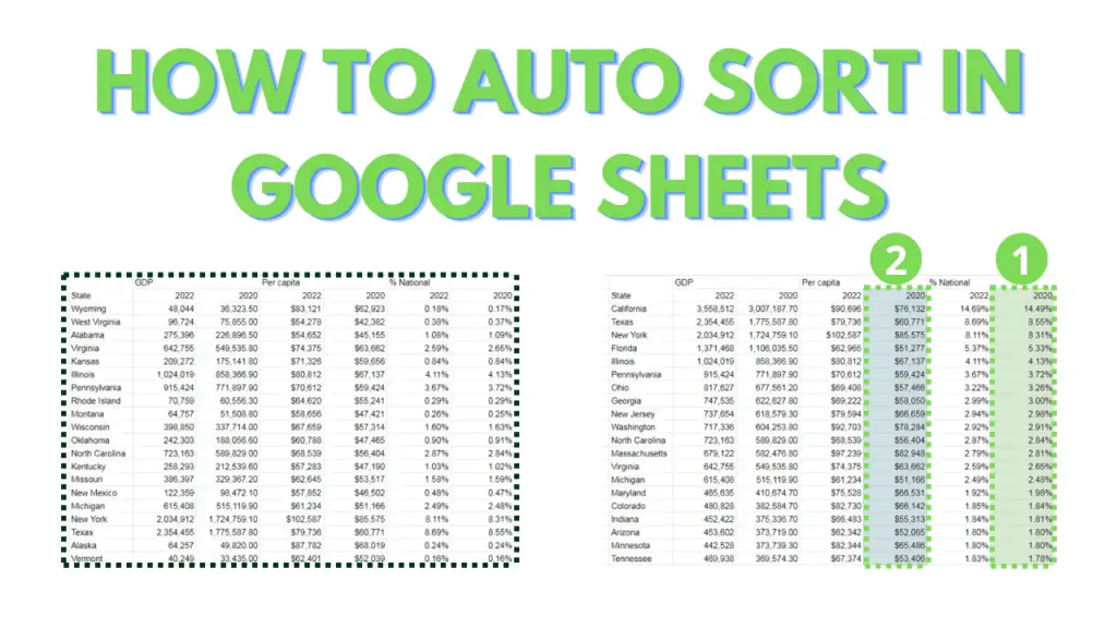
2. Identify the local index of the columns that you want to sort for in your range
3. Adjust the SORT formula by replacing “range” with the address of your range, “sort_column” with the index of the column, and “is_ascending” between TRUE and FALSE, or 1 and 0
4. (optional) Adjust the SORT formula with information on the optional pairs “sort_column2” & “is_ascending2”, “sort_column3” & “is_ascending3”, etc.
5. (optional) Use an array to display column headers above the sort results
   “={header_range;SORT(range, sort_column, is_ascending)}”

Auto-Sorting in Google Sheets YouTube Video Tutorial

SORT function Syntax in Google Sheets

The syntax for the SORT function is:

SORT(range, sort_column, is_ascending, [sort_column2, …], [is_ascending2, …])

The SORT Function Syntax elements explained

• range: the range of the data that you want to use the SORT function on (exclude headers)
• sort_column: the local index (numerical form) of the column that you want to sort, within the dimensions of “range”
• is_ascending: boolean value (TRUE, FALSE, 1, 0) to set whether the corresponding sort_column should be sorted in ascending order

Auto Sort in Google Sheets Tutorial

For this tutorial, I will provide a sample file that will have 2 worksheets.

The first worksheet contains 2 tables, organized in a way that demonstrates how to identify the range that you want to auto-sort.

The second worksheet contains a table with numerous columns that would demonstrate how to identify the index of columns for use in the SORT function.

You can make a copy of the file by accessing it through this link, then by clicking on “File” from the menu bar, then by clicking on “Make a copy”.

A dialog box should appear. Within it, you can provide a filename for the copy then click “Make a Copy”.

Step 1 – Identify the range that you want to automatically sort

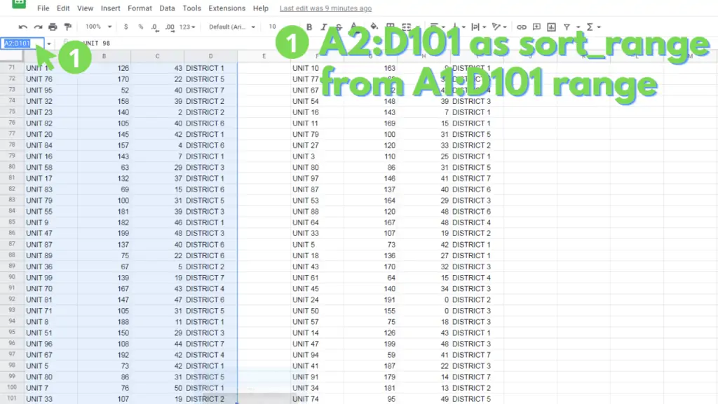
The first step in using Auto Sort in Google Sheets is identifying the range that you want to auto sort. In the example I provided in Sheet1, the address for the range of data would be “A1:D”.

However, given that the SORT function cannot disambiguate between headers and actual data, it’s best to exclude any header rows for your range. You should end up with a range address like this:

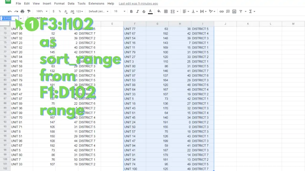
For the next table on range F1:I102, where there are 2 rows as headers, the range to sort would then be F3:I102, as shown below on the name box:

Step 2 – Identify the local index of the columns that you want to sort for in your range

The next step is finding out the local index of the column that you want to use for your SORT function. A local index is a number that represents the ordinal position of your column, within your range.

The first column in Sheet2 range “B2:K101” is column B, thus it has a local index of 1. Column C has 2, column D has 3, etc.

Identifying the local index for a column may be easy with a small range, but if you’re having trouble identifying them, you can use this formula:

=HLOOKUP([header],{ARRAY_CONSTRAIN([original_range],1,COLUMNS([original_range]));
SEQUENCE(1,COLUMNS([original_range]),1,1)},2,0)

Simply substitute [header] with the header title from your original range, then [original_range] with the address of the range that you want to sort, including the header rows, then enter it on any cell.

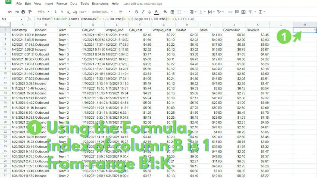
For context, the formula searches the local column index by matching the column header with a sequence of numbers.

The sequence of numbers starts at 1 and ends equal to the number of columns in the original range.

For example, let’s assume that you want to sort range B2:K101, using column C as the sort_range, the formula would then be:

Step 3 – Adjust the SORT formula by replacing [range], [sort_column], and [is_ascending] from “SORT(range, sort_column, is_ascending)”

With the information that you gathered from steps 1 and 2, you can now construct the SORT formula according to what you need.

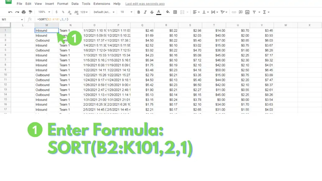
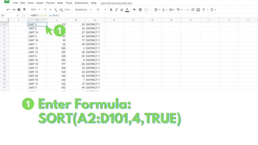
Let’s assume that you want to sort the data on range A1:D101 from Sheet1, which includes a single header row. We can now identify the [range] address to use as A2:D101.

Next, let’s assume that we want to use the data in column D as our [sort_column]. Since our range starts with column A, the local index of your [sort_column] is 4.

Next is the option of whether or not to use an ascending order for the sort column. You can type the following as your [is_ascending] choice: TRUE or 1 if you do, or FALSE or 0 if you don’t. For our example, let’s use TRUE.

Your formula and result should now look like this:

Optional Step 4 –  Adjust the SORT formula with additional pairs of [sort_column] and [is_ascending] values

The [sort_column2, …], [is_ascending2, …] parts of the SORT function denote optional pairs. They can be omitted, but to be included, a sort_column must pair with an is_ascending using the same number.

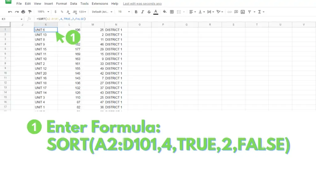
As an example, let’s assume that apart from sorting by column D in ascending order from the range A2:D101, we want to have an additional sorting column.

Let’s suppose that this is column B, which has an index of 2, and that we want it to be sorted in descending order.

Your formula and result should now look like this:

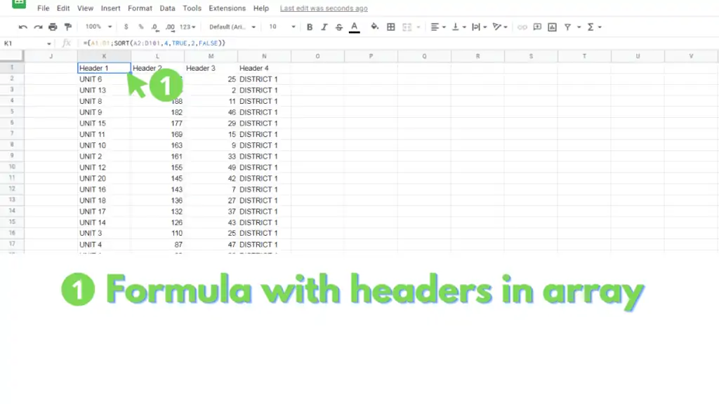
Optional Step 5 – Use an array to display column headers above the sort results

“={header_range;SORT(range, sort_column, is_ascending)}”

This is an optional step that adds a few components to your current formula, so that you will not need to manually copy and paste your column headers.

Simply replace “SORT(range, sort_column, is_ascending)” with the setup of your SORT formula, then replace “header_range” with the address that references your column headers.

For example, let’s assume that you want to sort the range A1:D101, through column D in ascending order.

The header_range will most likely be A1:E1, while the range to sort will be A2:E101. Column D will have a local index of 4, and to sort by ascending order, you will need to type in TRUE or 1 on the is_ascending part of the formula.

You should end up with a formula and result that looks like this:

Sort in Google Sheets Examples

Sort range A1:F15, which has 1 header row, by column C in descending order:
=SORT(A2:F15,3,0)

Sort range A1:F15, which has 2 header rows, first by column C in descending order, then by column F in ascending order:
=SORT(A3:F15,3,0,6,1)

Sort range B1:F15, which has 1 header row, by column C in descending order, while including the headers rows through an array:
={B1:F1;SORT(A2:F15,2,0)}

Frequently Asked Questions on How to Auto Sort in Google Sheets

Conclusion on How to Auto Sort in Google Sheets

First, identify what you’ll use as the “range” value. This is a range address reference, and should not include header rows. Next, identify your “sort_column” value. This is a local index of the column within your “range” address. Column E in range A2:F100 has an index of 5. Then dentify the sorting order that you want the SORT function to use on your “sort_column”. This is a boolean value: TRUE or 1 for ascending order, FALSE or 0 for descending order. Finally, substitute the values onto the formula with syntax: “SORT(range, sort_column, is_ascending, [sort_column2, …], [is_ascending2, …])”