How to Alphabetize in Google Sheets – The 3 Best Ways

Organizing data with the use of Google Sheets have never been so easy. Are you looking to arrange strings in your data in alphabetical order?

That is easy with the different sorting features and functions in Google Sheets. In the many years that I’ve worked with Sheets, I’ve discovered multiple ways to achieve this.

In this tutorial, I’m going to show you how to alphabetize in Google Sheets.

How to Alphabetize in Google Sheets

1. Select the range that you wish to alphabetize
2. Go to the ‘Data’ menu and then to the ‘Sort range’ sub-menu
3. Select ‘Advance range sorting options’
4. Tick the checkbox if your range has a header cell or row
5. Confirm the details and hit ‘Sort’

Read more about Alphabetize in Google Docs.

3 Different Ways to Alphabetize in Google Sheets

There are multiple ways to alphabetize in Google Sheets, but in this tutorial, I am going to tell you the three simplest ways to do so:

1. Alphabetize Using the Column Header Sort Options in Google Sheets

For situations where the dataset to be alphabetized is an entire column and without a header, the easiest and fastest way to alphabetize in Google Sheets is by using the column header sort options.

To do this, right-click on the column header and select ‘Sort sheet A to Z’ in the context menu that pops up.

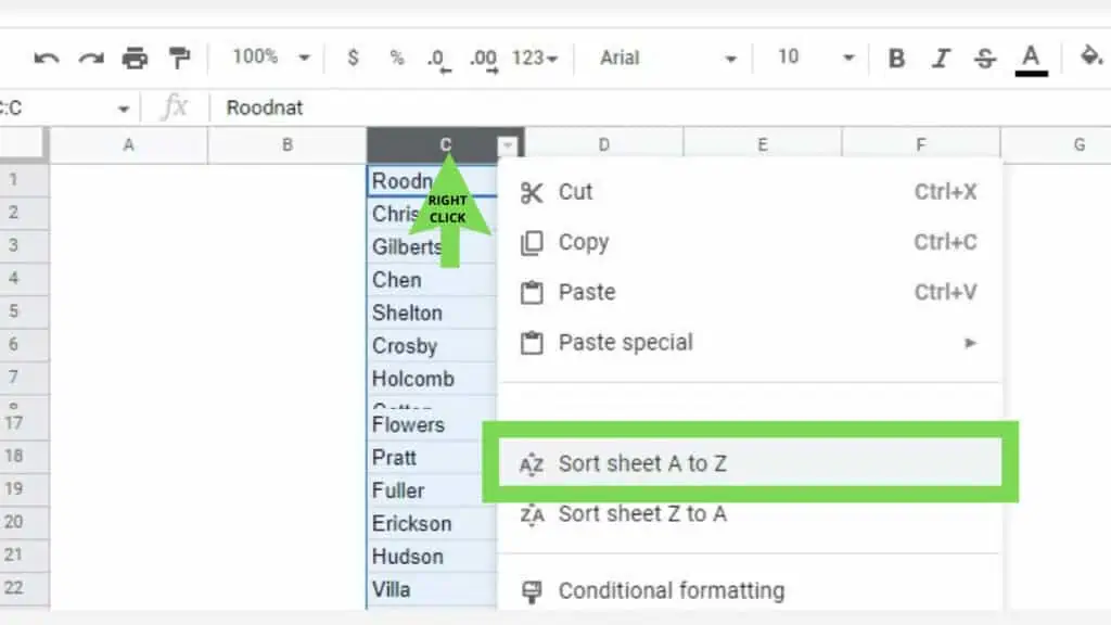
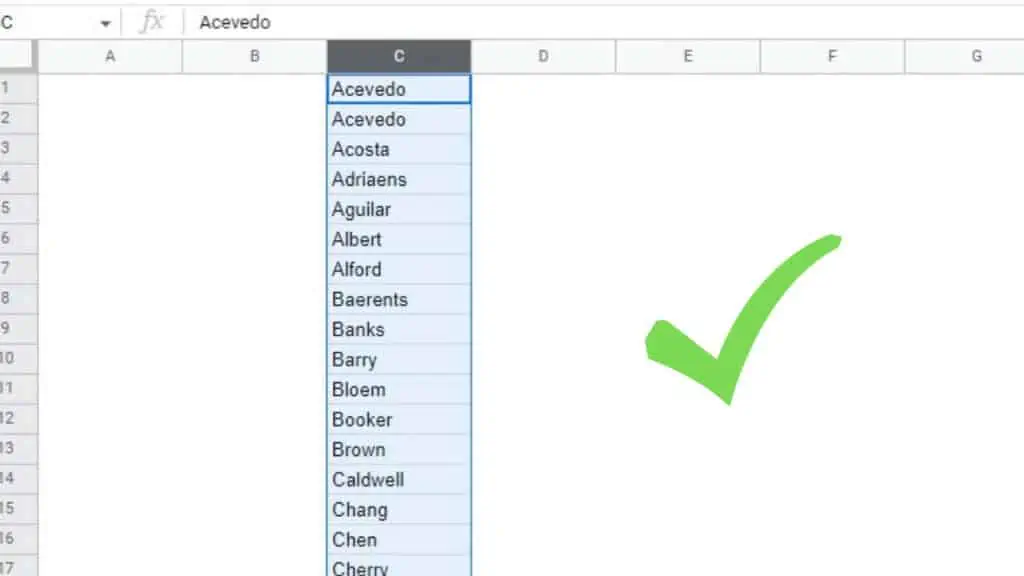
This should instantly alphabetize everything in that column. If you have other columns, they will not be alphabetized but will move accordingly dependent on the column that you’ve selected.

This method works for numerical values as well. The ‘A to Z’ in the options indicate that the sorting, other than being alphabetical, is also ascending (from smallest to largest).

2. Using the Data Menu Sort Options to Alphabetize in Google Sheets

Requires a few more steps but is more versatile than the first one, the Data Menu Sort method is a great way to alphabetize in Google Sheets.

To start, go to the ‘Data’ menu. Open up the ‘Sort range’ sub-menu and select ‘Advanced range sorting options’.

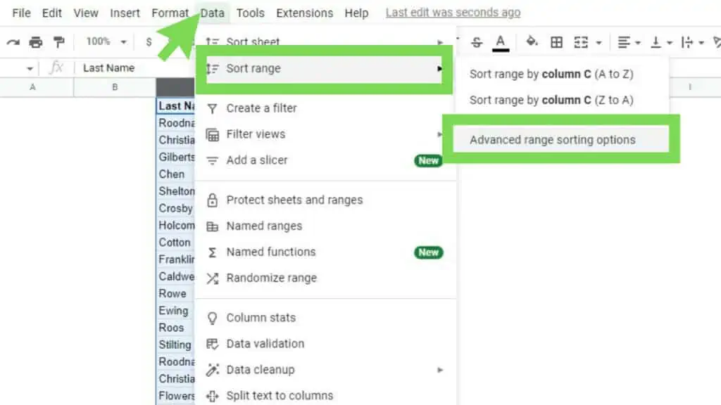
This will cause the ‘Advanced range sorting options’ window to show up.

Since the sample dataset that we’re working on has a header row, I ticked the checkbox beside 

‘Data has header row’. If your range doesn’t have a header, do not tick this checkbox.

This indicates if the first cell in the range is to be ignored or not.

Once you have confirmed that the options selected are correct, hit ‘Sort’.

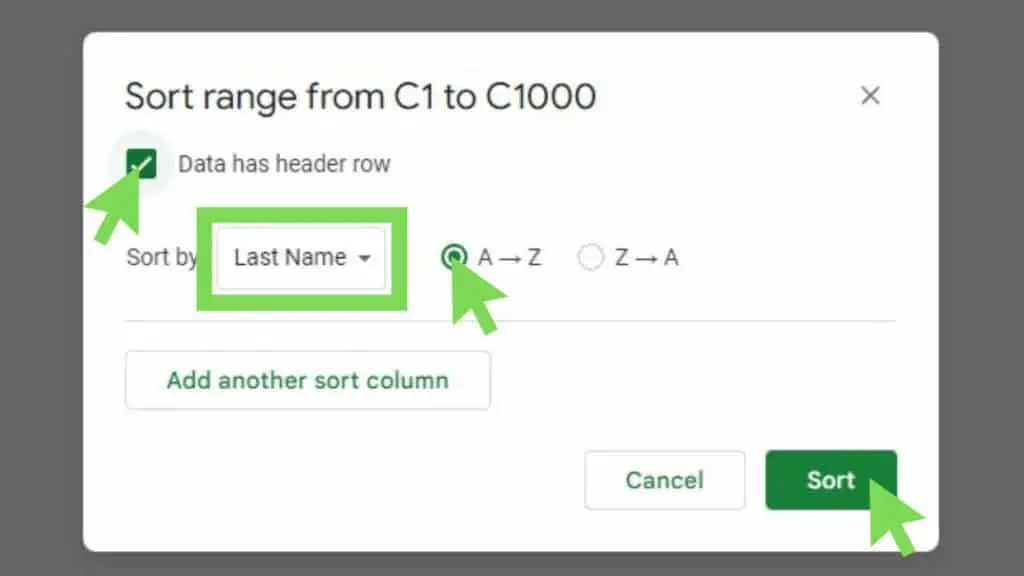
This will automatically alphabetize the dataset that I’ve selected and will also keep the header (Last Name) in its proper location.

There may be cases where you need to sort entire sheets based on a single column.

For example, I have a personnel datasheet that contains my employees’ information such as their last and first names, birthday, email address, and many more.

Using the ‘Sort sheet by column C (A to Z)’ option as seen above, where for example the employees’ last names are in column C, the whole sheet will be re-arranged following the last names being alphabetized.

This can also be done by using the SORT Function.

3. Using the SORT Function to Alphabetize in Google Sheets

Different than the first two, I can use the SORT Function to present the newly alphabetized data somewhere else without changing anything in the original data in Google Sheets.

Its syntax is as follows:

SORT(range, sort_column, is_ascending, [sort_column2, is_ascending2, …])

Where only the first parameter ‘range’ is required and the others are optional. If you don’t put anything on the sort_column parameter, the range will be the sort_column as well and for the third parameter, it will always be ‘ascending’ by default unless indicated otherwise.

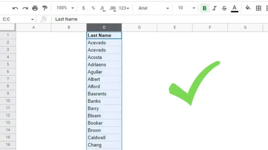
In the example below, there is a range (C:C) containing a list of last names. I used the SORT Function for it to be alphabetized and placed it in column E.

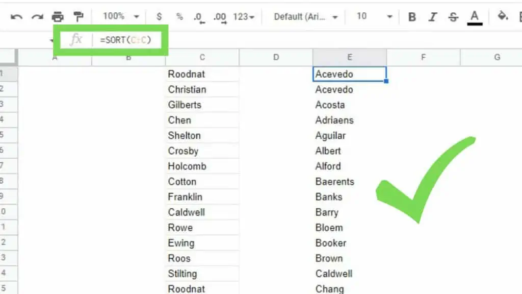
The downside here is that the SORT Function doesn’t have any provision to consider headers if your range has one. That said, it can be easily fixed by simply adjusting your range and just copying the header separately.

The best use of the SORT Function is that it can apply the capabilities of the ‘Advanced range sorting options’ but it can also be used in tandem with other functions and formulas.

It can be used with other functions such as UNIQUE or FILTER.

In the example below, I used the SORT Function on a huge dataset to alphabetize in Google Sheets.

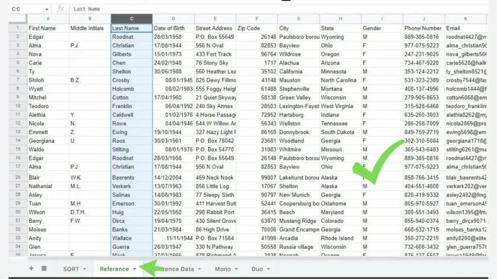
I started by identifying the range that I need to use as a reference in the ‘Reference’ sheet and I’ve also defined the column that will be used as the “sorting column”.

In the separate sheet, ‘SORT’, I’ve used the formula: 

“=SORT(Reference!A2:K,Reference!C2:C,TRUE)”

on cell A2 as I avoided including the headers from the dataset in Reference. To add the dataset from the ‘Reference’ sheet to the ‘SORT’ sheet, I used this formula:

‘=ARRAYFORMULA(Reference!A1:K1)’

and placed it on cell A1.

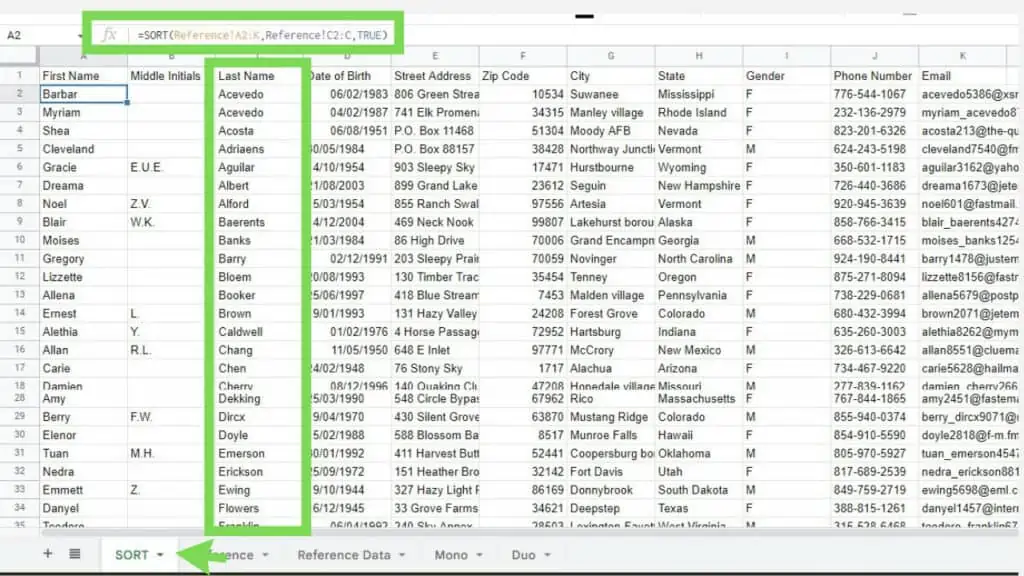
With this, I sorted the entire sheet based on each employee’s last name.

All the other columns from the same row followed through the sorting which makes sure that the data still matches each person accordingly.

This is how you alphabetize in Google Sheets. For best practices in manipulating huge datasets, it’s also best to learn how to unsort in Google Sheets.

Frequently Asked Questions about How to Alphabetize in Google Sheets

Conclusion on How to Alphabetize in Google Sheets

You can alphabetize in Google Sheets by selecting the range that you wish to alphabetize then going to the ‘Data’ menu and then to the ‘Sort range’ sub-menu. Select ‘Advance range sorting options’ and in the window that pops up, tick the checkbox if your range has a header, otherwise just confirm the details, and lastly, hit ‘Sort’.