In this tutorial, I will show you how to use the Google Sheets TEXT Function.
Like magic, Google Sheets automatically and correctly formats data when you input any value into a cell. That said, you may want to enter your data in another format than what was automatically assigned.
For these scenarios, the Google Sheets TEXT Function can save the day.
How to Use the Google Sheets TEXT Function
- Define the number that you wish to format
- Assign a format to be used, enclosed in double quotes
- Select a cell where you want the newly formatted number in
- Use this formula “=TEXT(number, format)”
- Hit ENTER or click on a different cell
TEXT Function in Google Sheets Video Tutorial
Syntax of the Google Sheets TEXT Function
TEXT converts a numerical value into a text that follows a format that you specify. It’s most useful in situations where you have numerical data that is in a format that is different than the one that you need.
The syntax of the Google Sheets TEXT Function is
=TEXT(number, format)
Where
- number – the numerical value either as a number, date, or time
- format – the pattern designed to reformat the numerical value enclosed in quotation marks if used directly on the formula; not enclosed in quotation marks if put in a cell
Below are some simple examples demonstrating the basic functions of TEXT.
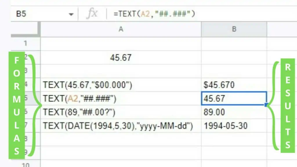
If you want to copy the formulas in the example, I’ve listed them down below:
- TEXT(45.67,”$00.000″)
- TEXT(A2,”##.###”)
- TEXT(89,”##.00?”)
- TEXT(DATE(1994,5,30),”yyyy-MM-dd”)
Rules and Format of the Google Sheets TEXT Function
The most important thing that you need to know when using the Google Sheets TEXT Function is the different formats that are used as the second parameter of TEXT.
As shown above, common symbols used in formats are “0” and “#”.
0 pushes zeros mandatorily if a numerical value has digits less than the format specifies.
Ex., TEXT(45.67,”$00.000″) produces $45.670.
Numerical values that have more digits to the right of the decimal point than the format parameter are rounded to the specified number of places.
Ex., TEXT(1.115,”00.00″) results in 01.12.
# is similar to 0 but does not force the display of zeros on either side of the decimal point.
Ex., TEXT(45.67″##.###”) produces 45.67.
Other rules:
- The format parameter of TEXT cannot contain the asterisk (*) symbol.
- TEXT cannot recognize the “? pattern”.
- TEXT does not work with fractional formats.
Next is a table containing the different format options for date and time values along with each one’s definition.
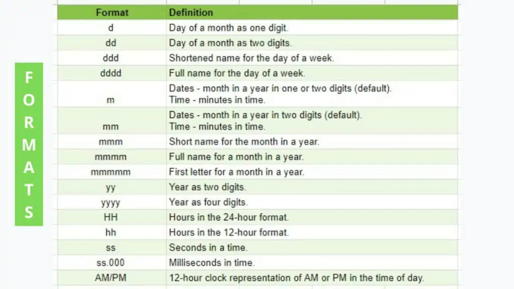
Depending on how you need your date and time values to appear, you may mix and match each format option here. Take note that repeating the exact same format option will result in the same value being repeated in the result of the Google Sheets TEXT Function.
Date and Time Examples of the Google Sheets TEXT Function
I’ve created a few examples to show some of the most used date formats and how they work.
Take note that for each example, a single format was written and that it doesn’t have quotation marks enclosing it. The formula for the 24 March 2021 is “=TEXT(B5,B3)” where B5 contains the numerical value which is “3/24/2021” and B3 contains the date format “dd mmmm yyyy”.
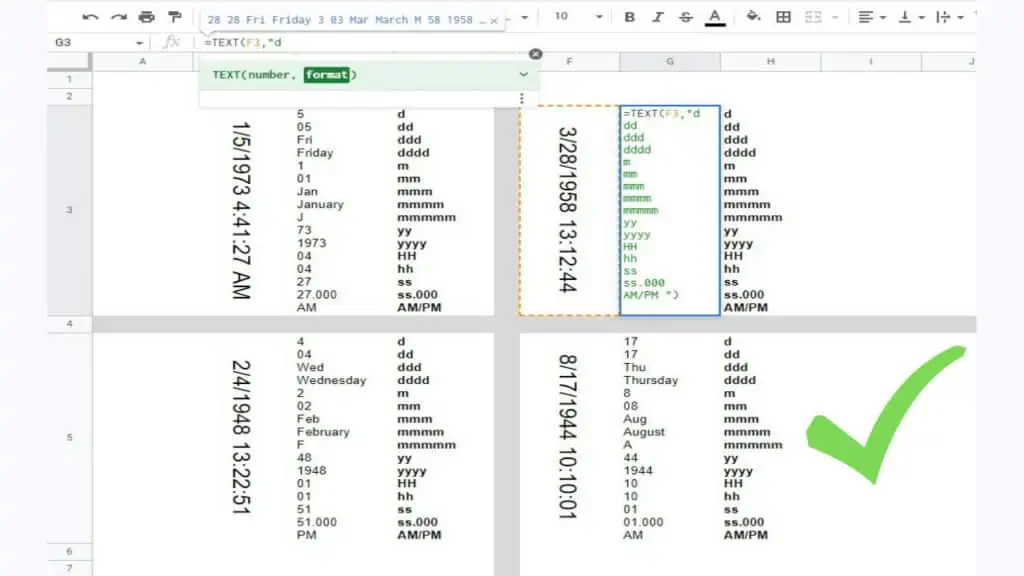
If I’m going to write the date format above inside the Google Sheets TEXT Function, it would look like “=TEXT(B5,”dd mmmm yyyy”)”.
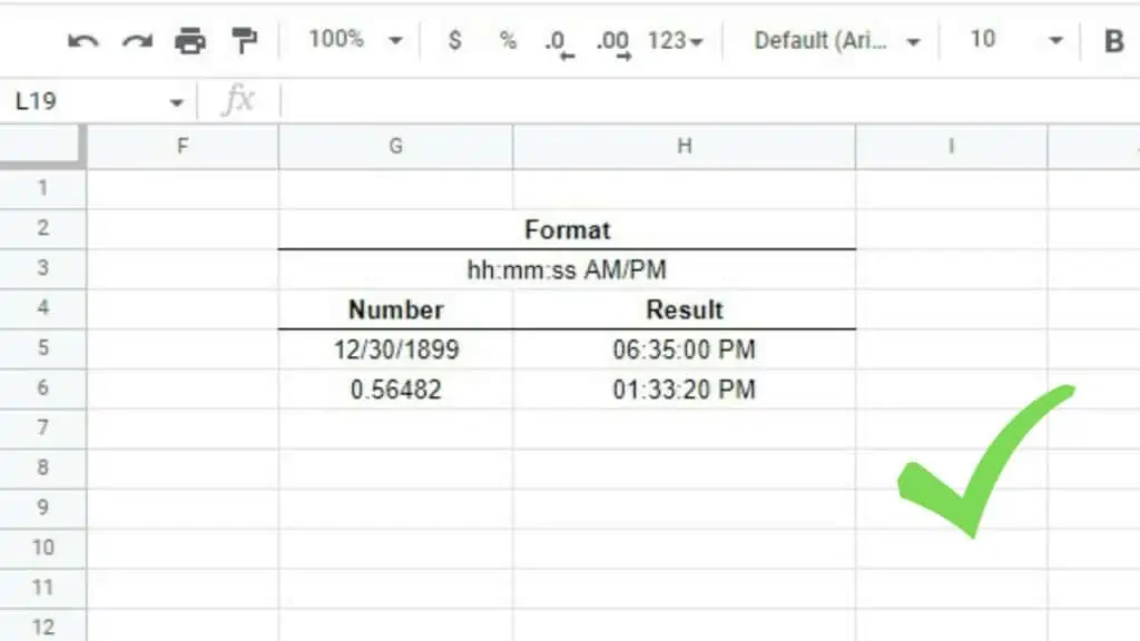
The example below is for time values.
And in this last example, I’ve shown what a combined date and time format looks like.
Aside from the date and time values, there are also other ways to use the Google Sheets TEXT Function. I’ve listed a few below.
Other Examples of the Google Sheets TEXT Function
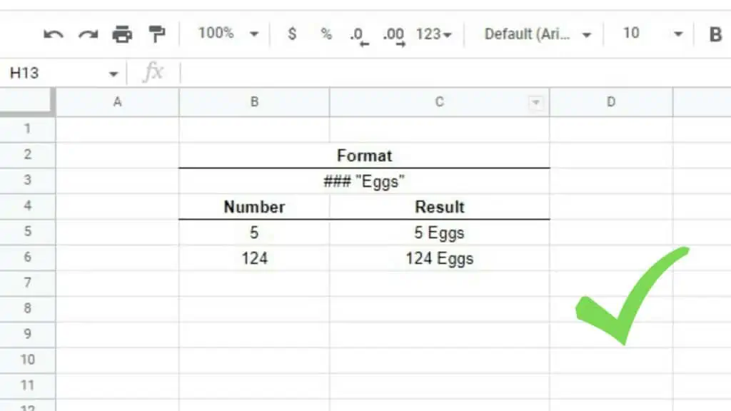
Another awesome way to use TEXT is to include strings that act as units for numerical values. Something like “pieces”, “grams”, or “meters” can be included as the output of the Google Sheets TEXT Function.
In the screenshot below there are two examples of amounts of eggs that I want to be displayed having the word “Eggs”.
To that, I simply need to use the format ### “Eggs”.
Other than knowing the right way to put in the string that will act as the unit description of your numerical value, it’s also important to identify when it is best to use a 0 or a #.
In the example below, since I used 0s in the format, it resulted in an awkward output like 028.100 Liters where most of the zeroes in this example are unnecessary.
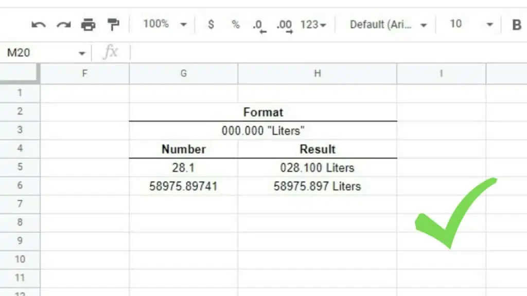
0 forces the output to have 0s for numbers with fewer digits depending on how many you’ve included in the format. This is often best used with currency denominations where the format should be “0.00” along with the currency symbol enclosed in quotation marks.
In the last example, you can see that I’ve inputted strings both before and after the numerical value. You can always adjust the format depending on how you need the output to look.
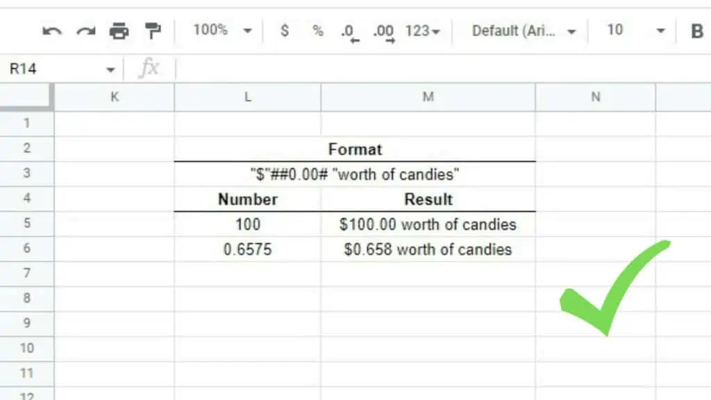
The important thing to remember here is that if you’re going to use strings in-cell references such as in the examples above, make sure to enclose them in quotation marks.
If you want to input special symbols such as the Euro sign or the degrees symbol, you may check out my other tutorials as well.
Frequently Asked Questions about How to Use the Google Sheets TEXT Function
How can I use the TEXT Function in Google Sheets?
To use the Google Sheets TEXT Function, you must follow the formula “=TEXT(number, format)”. Where the first parameter is the number that you wish to reformat and the second parameter, enclosed in double quotes, defines the format to be changed to.
Is there a different way to change formatting other than the Google Sheets TEXT Function?
Other than the Google Sheets TEXT Function, you may also use the menu option to change the formatting of a number. Just go to ‘Format’ and then ‘Number’ and you may use the formats listed there or the custom options at the bottom of the same list.
Conclusion on How to Use the Google Sheets TEXT Function
To use the Google Sheets TEXT Function, you must first define the number that you wish to format and then assign a format to be used, which will be enclosed in double quotes. Afterward, you must select a cell where you want the newly formatted number to be and use this formula “=TEXT(number, format)”. Lastly, hit ENTER or click on a different cell.

