In this tutorial, I will show you how to analyze data using multiple criteria with the Google Sheets SUMIFS Function.
It’s possible to have entire datasets in Google Sheets consisting of tens to hundreds of columns and rows depending on your needs.
Storing huge amounts of data can be all well and good until you need to get some analysis and interpretation done.
Despite Google Sheets having several functions that can help users take care of data analysis, even for multiple criteria requirements, it is often tempting to take the easy way out and just do things manually.
Unless you’re willing to work on it for weeks or even months, the Google Sheets SUMIFS Function can be the solution.
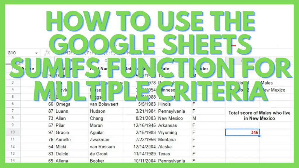
How to Use the Google Sheets SUMIFS Function for Multiple Criteria
- Identify the range with the values to be summed
- Define the ranges that will be checked against criteria
- Declare the criteria that will be the conditions for the ranges respectively
- Use this formula “=SUMIFS(sum_range, criteria_range1, criterion1, [criteria_range2, criterion2, …])”

3 Examples of How to Use the Google Sheets SUMIFS Function
Unlike SUMIF where there is only a single criterion to be checked and if a value meets the conditions it’ll be summed, the Google Sheets SUMIFS Function requires a value to meet all declared conditions before it is included as an addend.
The syntax of SUMIFS is
=SUMIFS(sum_range, criteria_range1, criterion1, [criteria_range2, criterion2, …])
Where
- sum_range – the range with the numbers to be added together
- criteria_range1 – the range where criterion1 will be checked against
- criterion1 – the conditions to be checked against criteria_range1
- criteria_range2, criterion2, … – [OPTIONAL] – set of criteria ranges and respective criterion to be checked against them
Below are some examples where I used the Google Sheets SUMIFS Function.
Example 1: Setting the First Example with Multiple Criteria
Compute the average sale per customer of each male sales agent in Arkansas who was able to serve 10 or more customers.
This scenario calls for the values in the Sales and Customers column to be added if each respective row meets the following criteria:
- Male – Gender column must have an M which is an acronym for Male
- Arkansas – State column must be Arkansas
- 10+ Customers – meaning the Customers column must have a value of 10 or higher
To compute this, I used the formula:
=SUMIFS(E:E,D:D,”M”,C:C,”Arkansas”,F:F,”>=10″)
As seen below.

To get the Average Sale, which is the Total Sales divided by Total Customers, I also need to compute the latter value.
Now, since I need to use the same conditions, I can simply copy the previous formula and just change the sum_range parameter to be the Customers column giving me the formula:
=SUMIFS(F:F,D:D,”M”,C:C,”Arkansas”,F:F,”>=10″)
As seen below.

Now that I have I can compute the Average Sale, which I did on the next screenshot.
Example 2: Minor Changes in Criteria
Comparison: compute the average sale per customer of each female sales agent in Arkansas who was able to serve 10 or more customers.
Unlike earlier where I simply needed to change the sum_range to find other values with the same set of criteria, I will now show you how easy it is to change an existing Google Sheets SUMIFS Function to reflect a different set of data based on criteria with minor changes.
The main difference in criteria here is that wanting to compare the average sale metric of males and females, I also needed to compute the numbers of the latter group.
To do this, I have to change “M” to “F” for the Gender column value in the formula giving me:
=SUMIFS(E:E,D:D,”F”,C:C,”Arkansas”,F:F,”>=10″)
and
=SUMIFS(F:F,D:D,”F”,C:C,”Arkansas”,F:F,”>=10″)
This gave me an overview of the comparison of Average Sale between Male and Female sales agents. Clearly showing that even though males, in general, have a higher total number of sales, females on the other hand are more efficient in terms of getting a higher number of sales per customer.

What if the minor change in criteria is on the State column?
Comparison: compute the average sale per customer of each male and female sales agent in Wyoming who could serve less than 10 customers.
Editing the earlier formula, I got:
=SUMIFS(F:F,D:D,”F”,C:C,”Wyoming”,F:F,”<10″)
I only need to edit the part in the formula where it says “Wyoming” instead of “Arkansas”.

Knowing how to manipulate the different Google Sheets SUMIFS Functions that you have to produce different perspectives or analyses of your data can be very useful.
Example 3: Different Analysis
Compute the average sale per customer of each male and female sales agent in Wyoming who could serve less than 10 customers.
This can be computed similarly to the earlier ones.
The formula for this will be
=SUMIFS(F:F,D:D,”M”,C:C,”Montana”,F:F,”<10″)
This is for the Total Hours for the first set of conditions.

The Served Meals is also summed for this example so I can compute for the Meals / Hour value which in this case is 7.
Next, I will compute the same values but for the Female group which can be seen in the next screenshot.

In doing so, I was able to get the values of 6 Meals / Hour for Females which is lower than for Males.
With this analysis, I was able to get an overview that males can be more efficient than females for stores located in Montana, for agents who worked for less than 10 hours.
Take note that the above analyses are just examples and are in no way comprehensive.
Depending on how you use the Google Sheets SUMIFS Function, it can serve as a precursor to a larger continuous set of research or can be a major indicator in itself as well.
After the analysis is done, it’s best to present the findings from the Google Sheets SUMIFS Functions through different graphs such as bar graphs or even pie charts.
Frequently Asked Questions about How to Use the Google Sheets SUMIFS Function for Multiple Criteria
How can I use the Google Sheets SUMIFS Function for Multiple Criteria?
To use the Google Sheets SUMIFS Function for multiple criteria you need to identify the sum_range. Next, define the ranges that will be checked against the criteria and declare the criteria that will be the conditions for each range. Finally, use this formula “=SUMIFS(sum_range, criteria_range1, criterion1, [criteria_range2, criterion2, …])”.
How many criteria can be used as parameters of the Google Sheets SUMIFS Functions?
ou can have as many as 127 pairs of criteria ranges and criteria when you use multiple criteria for the Google Sheets SUMIFS Function. Take note that it will be really difficult to reach this maximum number and have a working SUMIFS Function because every single condition must be met.
Conclusion on How to Use the Google Sheets SUMIFS Function for Multiple Criteria
To use the Google Sheets SUMIFS Function for multiple criteria you need first to identify the range with the values to be summed. Next, define the ranges that will be checked against the criteria and declare the criteria that will be the conditions for the said ranges respectively. Finally, use this formula “=SUMIFS(sum_range, criteria_range1, criterion1, [criteria_range2, criterion2, …])”.

