In this tutorial, I will show you how to use FOR LOOP in Google Sheets.
There are multiple ways of using Google Sheets with its vast functionalities. And depending on your requirements, there may be methods to approach some features that are better than the rest.
One of the methods that can be done is using the FOR LOOP technique. That said, it is often done through Google Scripts which can be much more complicated than desired.
How to Use FOR LOOP in Google Sheets
- Define the action to be looped
- Use the script format: “for ( var i = start_value; i <= end_value; i++ ){ [define the range] [select the range] [perform the action on the defined range] }”
- Declare necessary variables and steps

Using For Loop in Google Sheets
Using FOR LOOP in its purest sense means that you’ll be using Google Script and that is far from easy if you haven’t been using it already.
So other than the Google Script method of using FOR LOOP in Google Sheets, I also included other methods that I showed below.
1. FOR LOOP in Google Script
Looking at how FOR LOOP in Google Sheets work through a Google Script search isn’t as straightforward as it should be.
That is why I have created an example below where I detailed steps using FOR LOOP in Google Sheets.
In the example below is a list of names for an attendance sheet to that I need to add checkboxes.
I will show you how to do this by using a FOR LOOP in Google Sheets, which is through Google Script, to be precise.

Of course, the simple way to do this is just to simply select the range where the checkboxes will be added and insert said checkboxes.
But for this example, we’ll insert them through Google Scripts instead.

To go to Google Scripts, just go to Extensions > Apps Script. This will give you an empty default function in an Untitled Project.
The naming conventions won’t really affect how the script works, but it’s a good practice to rename them when you can.
The core of this Checkbox FOR LOOP Function is
for ( var i = start_value; i <= end_value; i++ ){ [define the range] [select the range] [perform the action on the defined range] }
Where
i – is an arbitrary variable to contain the counting stage
{body} – contains the range, how it is selected, and the action to perform. These can all be in a single argument.
It is best to know about the basics of Google Script to understand this further.
The arbitrary “i” serves as the “counter” of FOR LOOP in Google Sheets. The statements in the parentheses can be interpreted as “i” is equal to “start_value.”
As long as “i” is less than or equal to “end_value,” the {body} statement will run. For every instance that the {body} runs, the value of “i” will increase.
This means that if we have a start_value of 3 and an end_value of 22, the FOR LOOP in Google Sheets will run 20 times which starts from when “i” was 3 until it gets to 22 because of the “i++” statement. (You can try counting in your fingers from 3 to 22, and you’ll get 20.)
Checkout my entire script below:
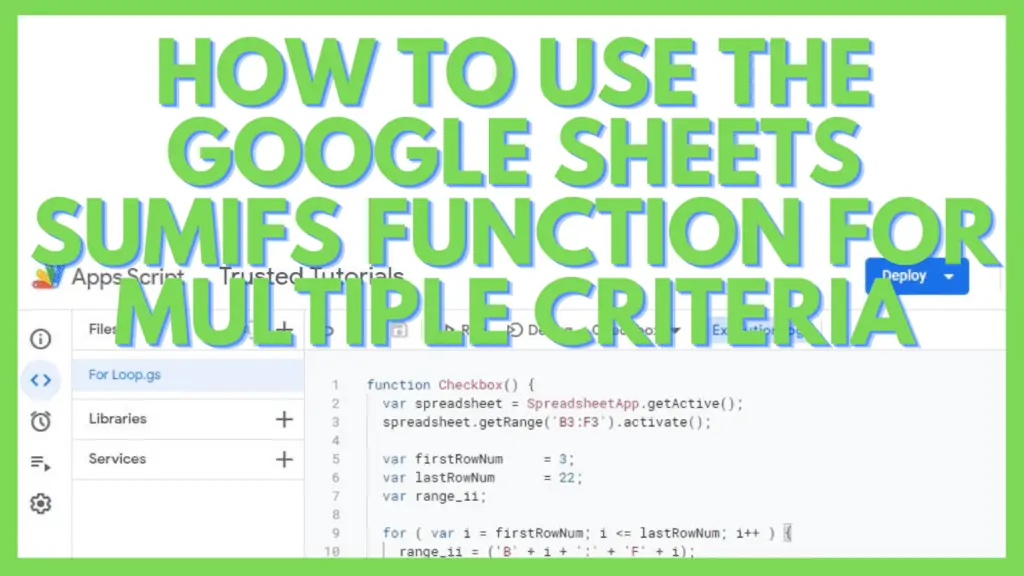
function Checkbox() {
var spreadsheet = SpreadsheetApp.getActive();
spreadsheet.getRange(‘B3:F3’).activate();
var firstRowNum = 3;
var lastRowNum = 22;
var range_ii;
for ( var i = firstRowNum; i <= lastRowNum; i++ ) {
range_ii = (‘B’ + i + ‘:’ + ‘F’ + i);
spreadsheet.getRange(range_ii).activate();
spreadsheet.getActiveRangeList().insertCheckboxes();
}
};
You can define anything in the body statement as long as it includes a target cell or range that is affected by the “i” variable.
This is crucial as this will make the actual loop work since the range changes from cell to cell, row to row, or column to column with every run.
Once you’re done with the script, just click on the diskette icon to save your Google Script project.

Next, click on the Run button.

If this is the first time that you will be running this saved version of the script, it will require authorization.
Click on ‘Review permissions’.

Next, click on your Google account.

Sometimes, Google will show a warning about verification as a precautionary measure.
Now, as long as you are confident of the script that you have created (or copied), just click on the bottom-most option where it says “Go to [project name] (unsafe)”.

Next, a confirmation window will appear. Hit ‘Allow’.

This will now run your script. If there are no errors, you will see in the Execution log the messages ‘Execution started’ and ‘Execution complete’.

I now have checkboxes in my sheet that were added using FOR LOOP in Google Sheets.

There are a lot of potential options to expand further the code that I used for this example.
Instead of manually setting the end_value of the FOR LOOP in Google Sheets, I could have instead created a function in the sheet or added some more lines in Google Script for the last row to be automatically detected.
Doing it that way would allow me to add or delete names, and the checkboxes will be adjusted accordingly.
2. FOR LOOP Via Conditional Formatting
Like with my other tutorials, I always prefer presenting alternatives to the fundamental way of using a function or feature like FOR LOOP in Google Sheets.
FOR LOOP works in a way where certain actions will be repeated repeatedly until the desired outcome or limit is reached.
There are multiple ways to reproduce FOR LOOP in Google Sheets without using Google Script.
I used the same dataset in the previous one for my next example, where I selected the entire column for the checkboxes minus the header rows. This time, we will use Conditional Formatting to apply the concept of FOR LOOP in Google Sheets.

Next, I inserted checkboxes in the entire range.

Now, I’m going to apply conditional formatting on the entire range. To do this, I just need to go to the Format menu and select Conditional formatting.

In the Conditional format rules window, with the entire “checkbox range” selected, I selected the ‘Custom formula is’ option. In there, I used the formula:
=ISBLANK($A:$A)
Where the A column contains the name in the sample list.
At the same time, in the ‘Formatting style’ section, I changed the Fill color and Text color to White which means that if the condition is met, the checkboxes will be white, rendering it invisible whenever there is no name in the respective cell in the A column.

This also means that whenever I need to add more names to the list, I simply have to type it in the A column, and the respective checkboxes in columns B to F will automatically appear.

This can be interpreted as a FOR LOOP in Google Sheets, where checkboxes will be added until the variable “i” matches the row value of the last name on the list.
And with this setup, whenever a name is added to the list, the row value also increases.
3. FOR LOOP by Using Functions and Other Features
Other than using Conditional Formatting – certain functions and features can work like FOR LOOP in Google Sheets as well.
For example, I created a Sales dataset with rows in chronological order.
I want to compute the total amount of sales, the number of sold items, and the average sale from October 5 up until a certain date.
In a FOR LOOP in Google Sheets, this will have October 5 as the start_value (date value) while the end_value will be the date that I will be defining.
To do this, I used the SUM, INDIRECT, and XMATCH Functions. This is the formula used to compute the Sales:
=SUM(INDIRECT(“B3:B”&XMATCH(G3,A:A)))
The XMATCH Function allows me to get the row number of the date that I selected which is in G3, while INDIRECT provides a cell reference covering the sales from October 5 until that date. SUM then adds all the sales covered by the included dates.

For a more convenient way to select dates, I used Data Validation. This can be accessed through the Data menu. You need to mention the data range here, and it will show up as a drop-down list on the cell you selected.

This method can also be applied to compute the total number of sold items within a certain date range by changing the constant cell reference address of the INDIRECT Function from “B3:B” to “C3:C”.

Google Script is so much more powerful and versatile than Google Sheets but using it is so much more complex as well. That said, if you can use FOR LOOP in Google Sheets with a Google Script, that’s awesome!
But if you cannot, like the majority of Google Sheets users, I suggest that you stick to more common features and functions in Google Sheets, like the IF Function.
The most important thing to know if you want to apply FOR LOOP in Google Sheets is that you understand what you need so that you can better find out how you can get it, whether through Google Script, Conditional Formatting, or other functions and features.
Frequently Asked Questions about How to Use FOR LOOP in Google Sheets
How can I use or apply the logic of FOR LOOP in Google Sheets?
You can use or apply the logic of FOR LOOP in Google Sheets by doing it in Google Script as “for ( var i = start_value; i <= end_value; i++ ){ [define the range] [select the range] [perform the action on the defined range] }”. You can also use Conditional Formatting, functions, or internal features.
Can I copy a script with FOR LOOP in Google Sheets and use it on my own worksheet?
You can use FOR LOOP in Google Sheets that was copied from somewhere else on your worksheet as long as you can properly modify the ranges and variables mentioned in that script to fit the data that you have in your worksheet. Take note of sheet names and cell references.
Conclusion on How to Use FOR LOOP in Google Sheets
You can use FOR LOOP in Google Sheets by defining the action to be looped in the script format: “for ( var i = start_value; i <= end_value; i++ ){ [define the range] [select the range] [perform the action on the defined range] }”. Then, declare the necessary variables and steps for the entire script.

