Do you have a large data set and you want to find a certain piece of text within it? I know from personal experience that trying your luck with scrolling or using CTRL + F just isn’t efficient anymore.
After several years of working in Google Sheets, I’ve discovered how to use the Google Sheets FIND Function.
In this tutorial, I’m going to explain how to use the FIND Function along with some practical examples of how to use it.
How to Use the Google Sheet Find Function
- Identify the ‘search_for’ parameter
- Define the ‘text_to_search’ either as the actual text or cell reference
- If necessary, assign a value to the ‘starting_at’ optional parameter
- Use the formula: “=FIND(search_for, text_to_search, [starting_at])”
How to use the FIND Function in Google Sheets
In strings, there is a predefined positioning depicted by numbers from left to right. With 1 marking the first character on the left and will go as high as the total number of characters for the position of the rightmost character.
The FIND Function lets you search a text for the specific position of a piece of text. Its syntax is as follows:
=FIND(search_for, text_to_search, [starting_at])
The ‘search_for’ parameter indicates the actual text that you’re looking for or the reference to a cell containing said text.
The ‘text_to_search’ parameter defines where you’re trying to find the search_for text. It can be a longer string or the cell reference for it.
The ‘starting_at’ optional parameter lets you define where the search will start. Putting in a value for this parameter lets you skip a number of characters from the left. This is particularly useful for URLs where, for example, you don’t want to include the part “https://” or “www.”.
Below are some applications of the FIND Function in Google Sheets.
Main Feature of the FIND Function
The most basic of all the features of the FIND Function is to literally use it for finding specific texts within larger texts for different purposes.
One example of this is when you have a dataset of people’s information where you want to see who, from among the list, was born in 1944.
For that, we need to set the ‘search_for’ parameter of the FIND Function to “1944” and use the references of the cells containing birthdays.
We’re using the formula “=FIND(“1994”,E2)” for the example below and copy it to the rest of the column.
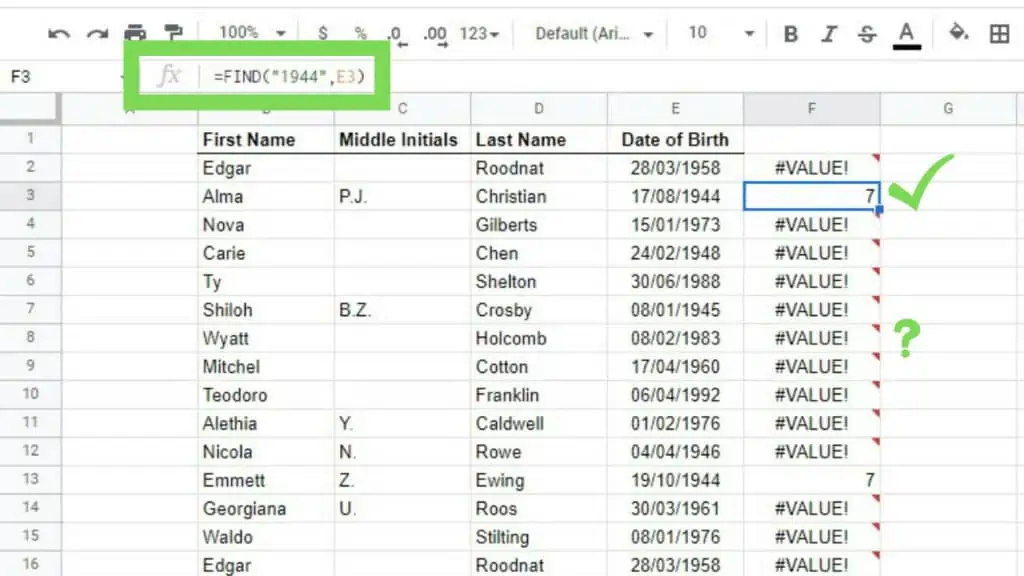
The downside of the FIND Function is that if it doesn’t find the text that it’s looking for, it will return an error. A quick solution to this is to simply add the IFERROR function.
To do that we just need to edit our initial formula to “=IFERROR(FIND(“1994”,E2))” and copy it to the rest of the column.
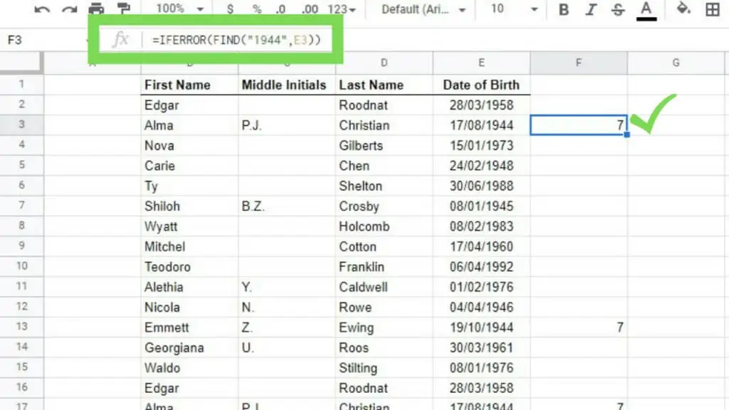
As you can see, I’ve set it up in such a way that if the FIND Function returns an error, the IFERROR Function will return a “blank”.
Now we know in this example that at least three people were born in 1944 with the number 7 indicating the position of “1944” in the DD/MM/YYYY format of the birthdates.
With the IF Function
Another application of the FIND Function is by using it with the IF Function. In doing so, we will not be limited to the results of the FIND Function where it only returns a number indicating the position of the ‘search_for’ parameter.
With the IF Function, we can take advantage of the FIND Function returning any number as confirmation that the cell being checked contains the ‘search_for’ parameter, regardless of position.
To better explain this, here’s an example below:
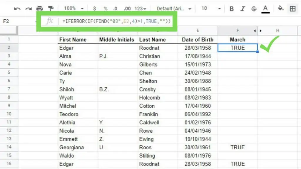
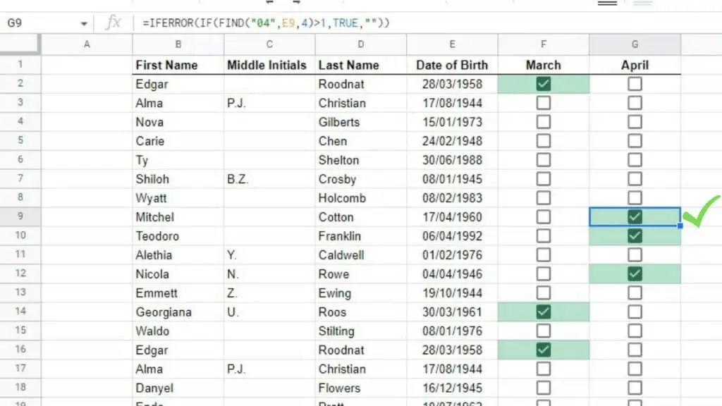
Using the same dataset earlier, I wanted to see which of these people were born in March so I used the formula: “=IFERROR(IF(FIND(“03″,E2,4)>1,TRUE,””))” and copied it down.
We can also do the same when looking for people born in April by changing the ‘search_for’ parameter of the FIND Function from “03” to “04”.
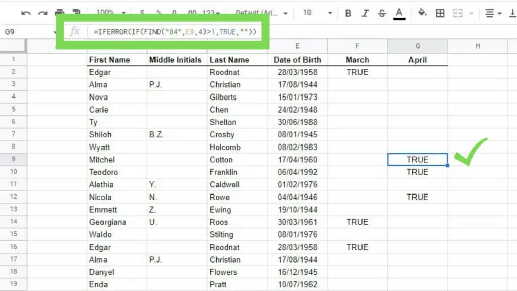
The TRUE shown in columns F and G indicates which rows contain information on people born in March and April, respectively.
Although as it is it can already be more useful and easier to locate people born in March and April, I’ll be showing you how to make this presented even better with checkboxes.
First, select the cells where you want the checkboxes to be. Then go to the ‘Insert’ menu, and select ‘Checkbox’.
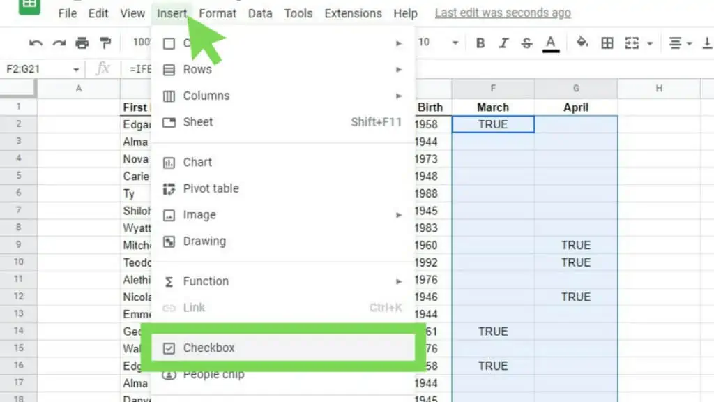
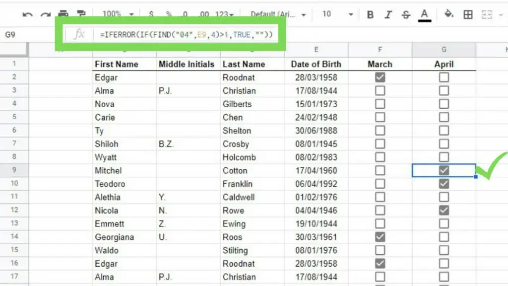
This will automatically put in checkboxes which will be ticked for cells with the value “TRUE” and remain unticked for cells with the value “FALSE”.
The last thing that you can do here is to apply Conditional Formatting. This is not necessary anymore but in the biggest datasets, conditional formatting helps users navigate through data.
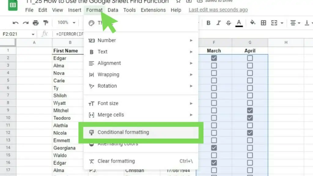
To do this, select the range to be formatted. Then go to ‘Format’, and select ‘Conditional formatting.
In the ‘Conditional format rules’ windows, change the rule to ‘Text is exactly’ and put in ‘TRUE’ as its value. You can change the ‘Formatting style’ to your preference if you want to. Then hit ‘Done’.

Aside from having the checkmark, it becomes even easier to spot data with conditional formatting applied to it.
Another way to do this is to assign conditional formatting to the columns separately. In doing so, you can create 2 distinct rules and have different colors for March and April.
Conditional Formatting in Google Sheets
Aside from using the IF Function where you can apply conditional formatting to its results, you can also use the latter straight up with the FIND Function.
To do this, we’re going to use the ‘Custom formula is’ feature of conditional formatting.
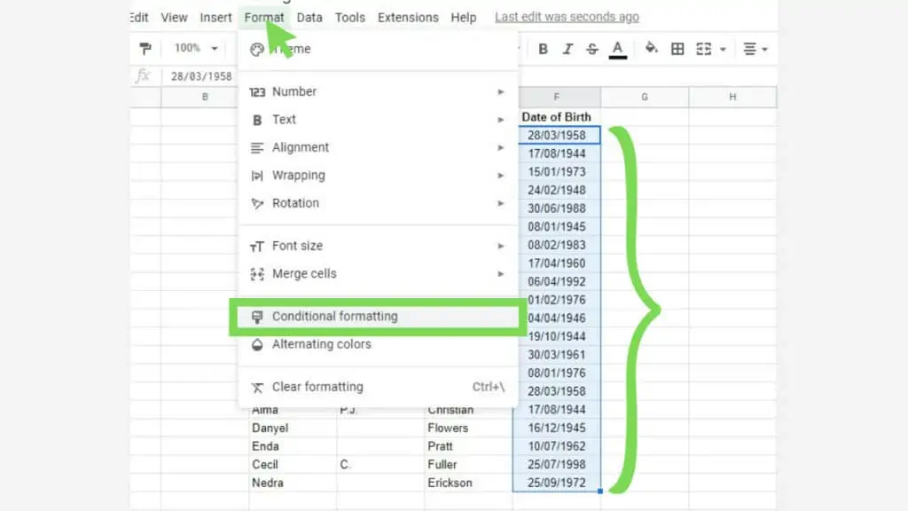
First, select the range that you want to apply FIND + Conditional Formatting to. Then go to ‘Format’ and select ‘Conditional Formatting’.
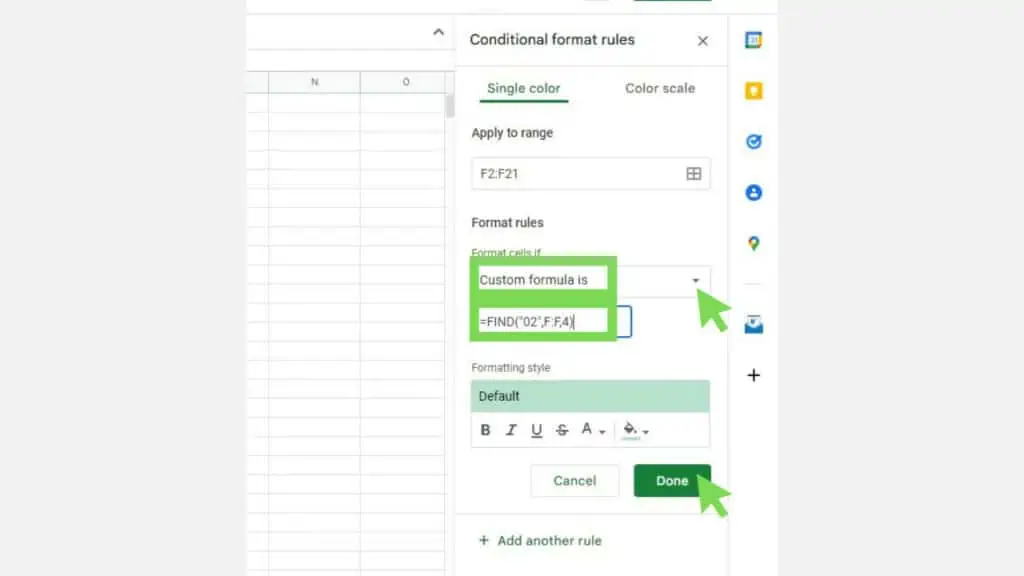
In the ‘Conditional format rules’ window, change the ‘Format cells if…’ to ‘Custom formula is’. In the field below it, enter the formula “=FIND(“02”,F:F,4)”.
The formula indicates that I wanted to find the string “02” which signifies February, on the range “F:F”, which covers our sample range “F2:F21”, and it should begin on the 4th character taking into consideration the DD/MM/YYYY syntax of the birthdates.
Now, without additional formulas or columns, we can identify the dates that fall in February.
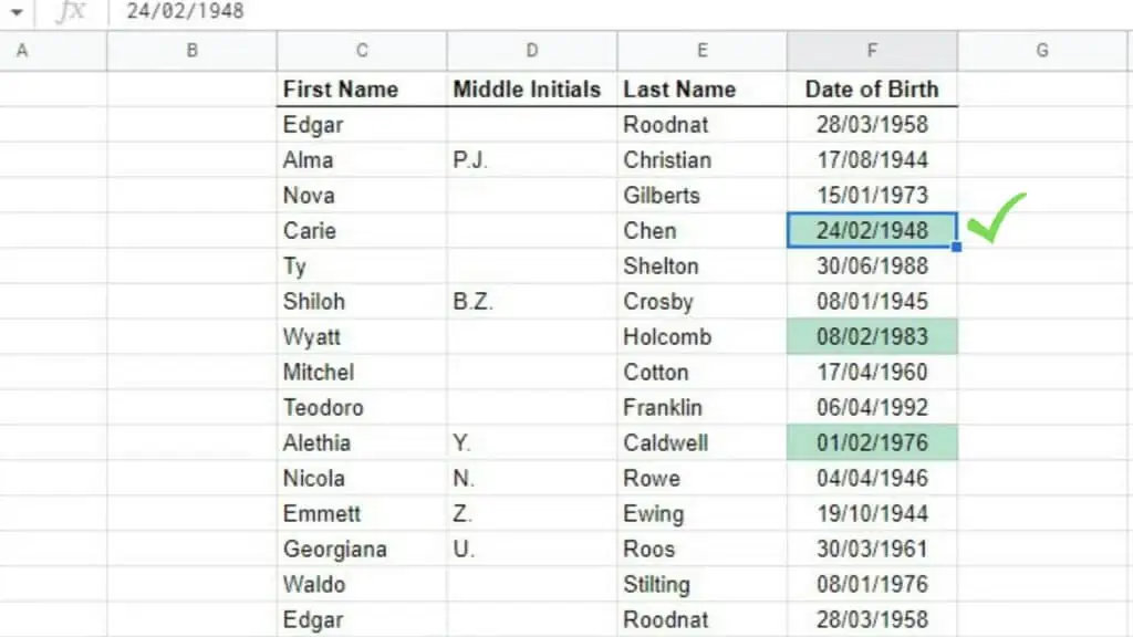
Caption: Birthdays falling in the month of February are highlighted
These are some of the ways I often use the FIND Function whenever I work on Google Sheets.
Frequently Asked Questions about How to Use the Google Sheets Find Function
Why is the FIND Function in Google Sheets not finding a text in a certain string even though it’s definitely there?
The most common issue with using the FIND Function is that it is case-sensitive. If you want to keep using the FIND Function, make sure that your case usage is correct. Otherwise, use the SEARCH Function instead.
How can I prevent the FIND Function in Google Sheets from always returning an error value?
To avoid error values being returned by the FIND Function in Google Sheets, simply encase FIND with the IFERROR Function. By default, doing this will simply return a blank for FIND error outputs
Conclusion on How to Use the Google Sheets Find Function
To use the Google Sheets Find function decide on the ‘search_for’ parameter and the ‘text_to_search’ parameter either as actual text or a cell reference. If necessary, assign a value to the ‘starting_at’ optional parameter. The find formula is: “=FIND(search_for, text_to_search, [starting_at])”.

