In this tutorial, I will show you how to create a Drop-down List in Google Sheets Step-By-Step.
Drop-down lists are categorized as a type of “Data validation” in Google Sheets. You can set up the elements within this list through the use of a list separated by commas, a range that is turned into a list, or custom formulas that output lists.
Finally, it is good to remember that a drop-down list in Google Sheets acts like a pseudo search bar that updates your remaining choices depending on what you have already typed.
How to Create a Drop-Down List in Google Sheets
To create a Drop-down List in Google Sheets:
- Select a cell or range
- Click on “Data” from the “Menu bar” then select Data Validation
- Choose between “List from a range” and “List of items” in the drop-down beside “Criteria”
- Select a range by clicking the “Table” icon (4 cells with thick outer borders) or enter a formula on the field
- Enter a list of items separated by a comma on the field
- Set up additional options besides the “On invalid data” and “Appearance” sections
- Select between “Show warning” or “Reject input” radio buttons
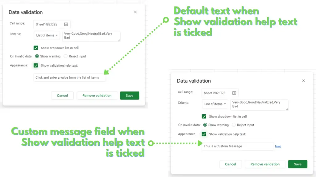
- Tick “Show validation help text:” checkbox then enter a custom error message
- Open the drop-down list then select your choice
Dropdown in Google Sheets Video Tutorial (Step-By-Step)
Dropdown List in Google Sheets Step-By-Step Instructions
Step 1 – Select a cell or range in Google Sheets
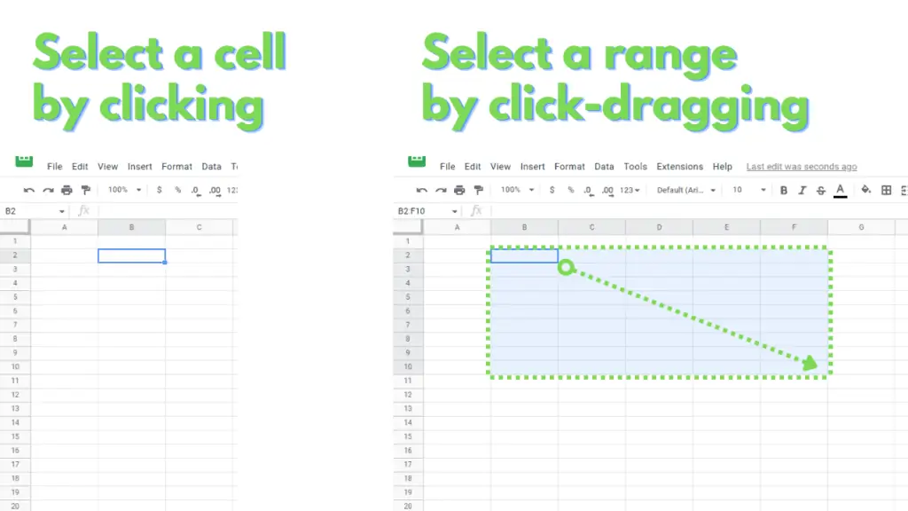
Our first step involves selecting a cell or a range to turn into a Drop-down List.
You can select a cell by clicking on it, while you can select a range by click-dragging from the first cell (top and leftmost) to the last cell (bottom and rightmost) of your range.
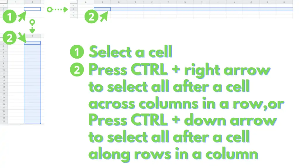
You can also select a range within a single row or column, after a certain cell in the row or column.
To do this across a row, click on the first cell that you want to select, then press CTRL + Shift + either left or right.
Likewise, press CTRL + Shift + either up or down if you want to select within a column.
To select a whole row or column, you can click a Column Letter or Row Number, or you can select multiple Columns or Multiple rows by click-dragging from one Column Letter or Row Number to another.
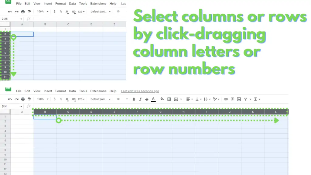
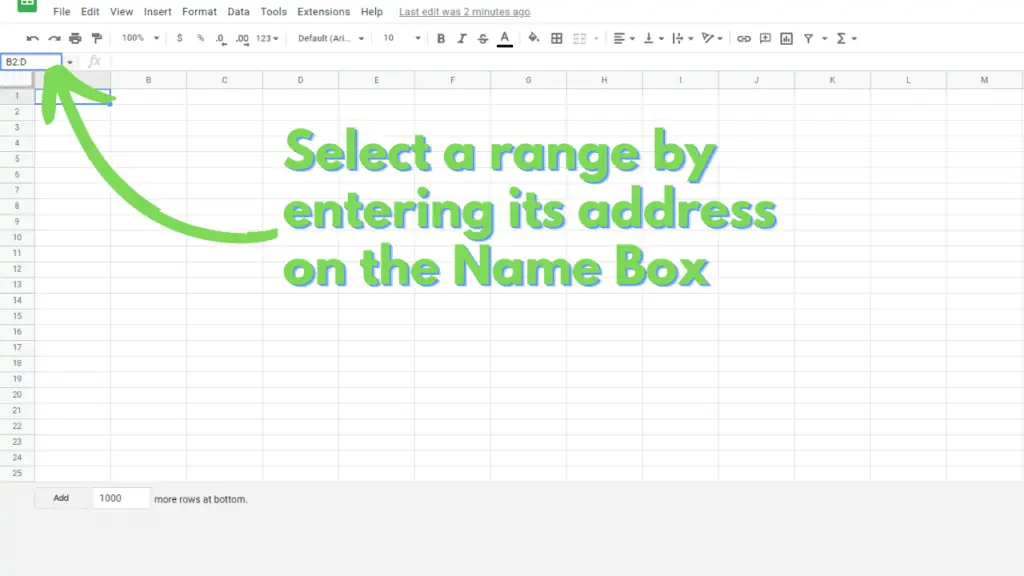
You can also select a range by entering its address in the “Name box”.
Step 2 – Click on “Data” from the “Menu bar” then select Data Validation
Once you have selected the cells or ranges, you can turn them into Drop-down Lists by clicking on “Data” from the “Menu bar”, then by clicking Data Validation.
This should open the “Data validation” dialog box that would look like this:
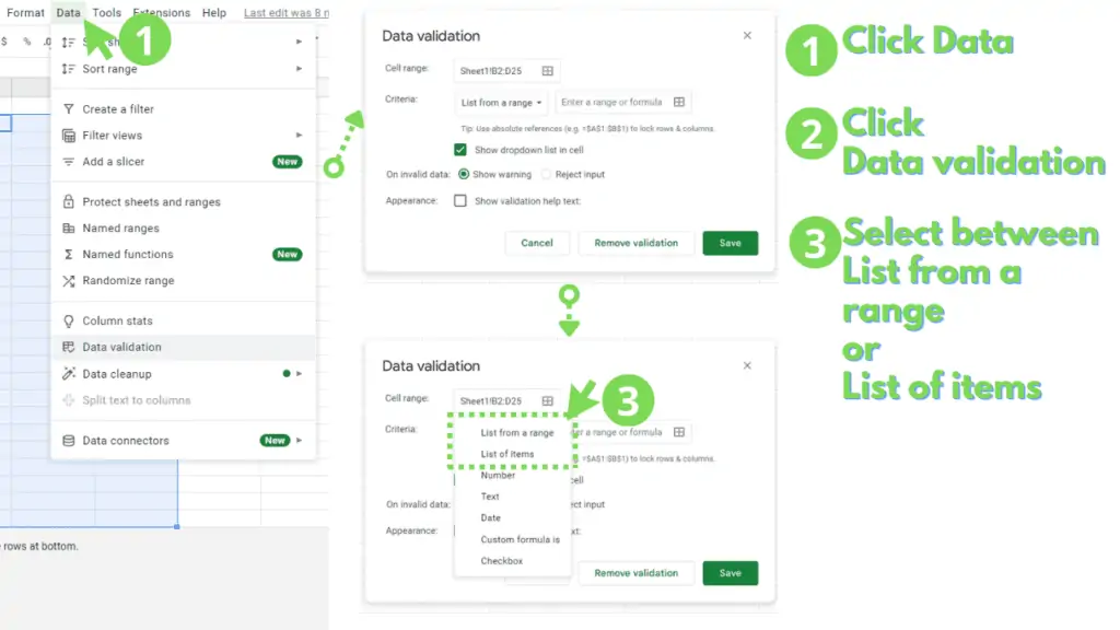
From here, you can select either “List from a range”, or “List of items”.
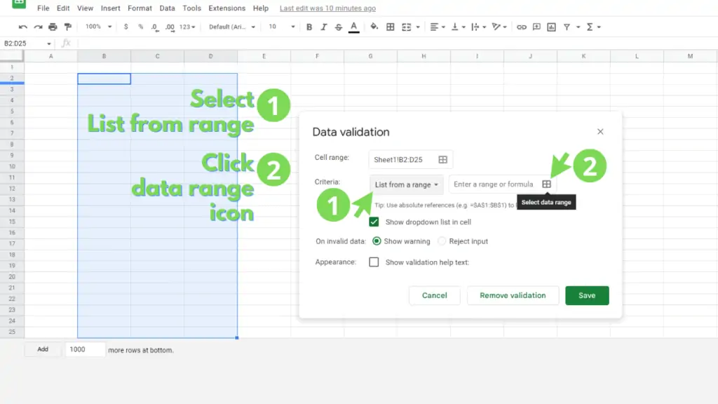
Step 3 – Choose between “List from a range” and “List of items” in the drop-down beside “Criteria”
If you chose “List from a range” back in step 2, you will need to provide the range by either typing in the range address to use on the blank field, or by clicking the “Select data range” button to the right of the field.
For this option, you can also select Named Ranges for your range.
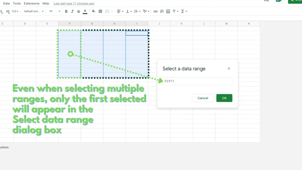
The latter will open up the “Select data range” dialog box that identifies your first selection’s address.
And while it’s possible to select multiple ranges (CTRL + click-dragging), only the first selection’s address will be returned.
This rule is consistent even if a subsequent selection is contiguous with the first selection.
If, however, you chose “List of items” back in step 2, you will need to manually enter the values you want on the field labeled “Enter items separated by a comma” using this syntax:
“[Item 1],[Item 2],[Item 3]”
Note that for each item to be recognized as a single entry in this field, they have to be “terminated” by a comma.
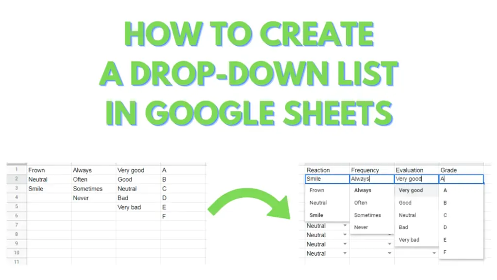
For example, to create a drop-down that contains “Very Good”, “Good”, “Neutral”, “Bad”, and “Very bad”, you must enter them in the field like this:
“Very Good,Good,Neutral,Bad,Very Bad”
Step 4 – Set up additional options besides the “On invalid data” and “Appearance” sections
There are additional options that you can select for a drop-down list in Google Sheets. You do this through the “Data validation” dialog box.
The first one is the option to either allow a user to enter a value that is not specified to be a part of the list that was set up or to restrict them from doing so.
The former will generate an error warning that will appear as a tooltip on the errant cell, while the latter will open a dialog box and reject the input.
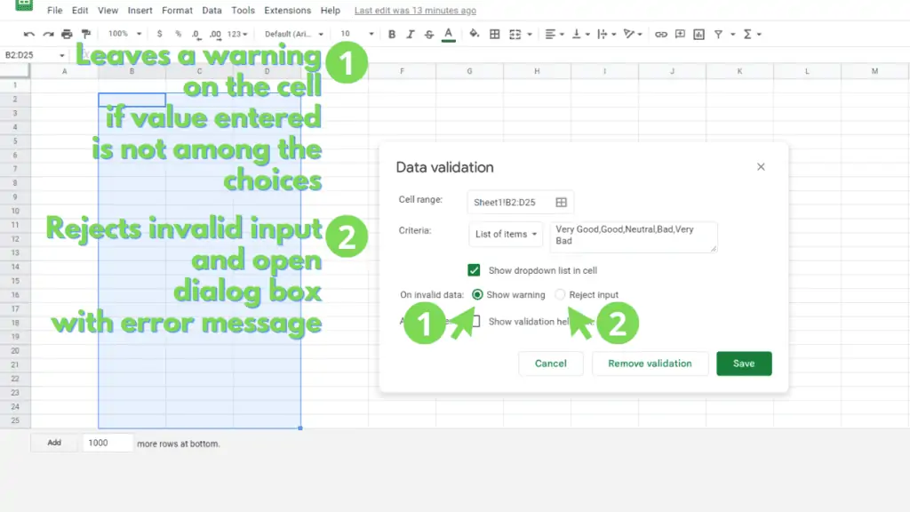
The second option is to specify a message to show on the dialog box when the drop-down list is set to “Reject input” and an invalid entry is provided for the cell.
These options don’t have to be customized at the initial creation of a drop-down list, as you can access them at a later time by selecting the cells, and accessing the “Data validation” dialog box.
Once satisfied with how you’ve set up your drop-down list, click the “Save” button.
Step 5 – Open the drop-down list then select your choice
Finally, we will explore several methods you can use to enter or select a value from a drop-down list.
To access the drop-down list for a cell, you can either click on the downwards-pointing arrow at the right of the cell or double-click the cell.

Once the drop-down list is active, the cell itself functions as a “smart” search field.
This smart search field is case-insensitive and will narrow down the list depending on what you have typed on the cell so far. It even highlights partial matches of your entry!
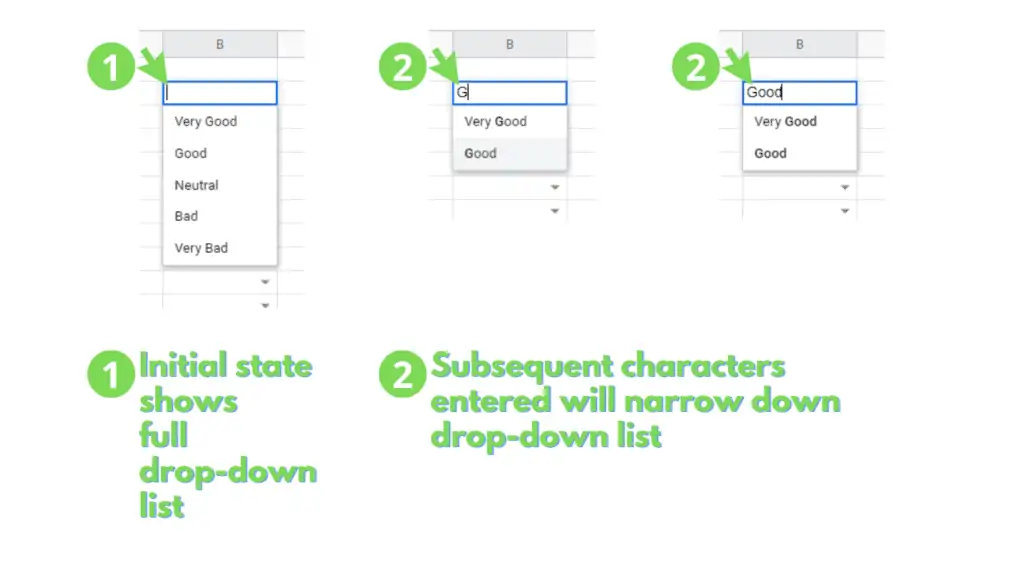
From here, you can click on your choice, or press the up and down arrows to shuffle through the choices before finally pressing the enter key.
You now know how to create a Drop-down List in Google Sheets.
Read about how to do an organizational chart in Google Sheets next.
Frequently Asked Questions on How to create a Drop-down List in Google Sheets
Is there a way to add leading or trailing spaces for items when using the “Items on a list” option in Google Sheets?
You can add leading spaces to an item by entering an apostrophe before any number of spaces. To get an item to show up as “ a”, you need to enter an apostrophe, followed by a space, followed by the letter “a”, then terminated by a comma. This is a workaround on the limitations of the option. On the list and the formula bar, it will explicitly show the apostrophe, but if that very same entry on the list is selected, the cell will return a value without the apostrophe.
Can I copy an existing drop-down list to apply to a range in Google Sheets?
You can copy a cell that’s set up as a drop-down list by first selecting it, then by pressing either CTRL + c or the copy button, then by selecting a cell, range, or selection of ranges. The destination ranges do not have to be contiguous for this method.
Conclusion on How to create a Drop-down List in Google Sheets
To create a drop-down list in Google Sheets, select which cells you want to convert into a drop-down by clicking a cell, or by click-dragging a range, column letter, or row number.
Next, click on “Data” from the menu bar and click “Data validation”.
In the “Data validation” dialog box, choose between “List from a range” or “List of items” in the drop-down for the “Criteria” section. For the former, select a range after clicking the “Table” icon on the right, or enter a formula on the field. For the latter, enter the values, separated by commas, in the text box.
Set up additional options by choosing between the “Show warning” or “Reject input” radio buttons. Then tick the “Show validation help text” checkbox and enter a custom error message in the provided field. Finalize the setup by clicking on the “Save” button.
Next, access the drop-down list of a cell by clicking the arrow on its right, or by double-clicking the cell.
Finally, click on your choice from the list, or partially enter a text in the cell to narrow down the choices, then select your choice.

