How to Use COUNTIF in Google Sheets – Read This

Do you have an inventory report with thousands of cells and you want to know which items are nearly out of stock? Did you realize that filtering and sorting just aren’t cutting it anymore?

The IF Function is one of the most useful functions in Google Sheets. One of its variants, the COUNTIF in Google Sheets can solve your problem.

In this tutorial, I am going to show you how to use COUNTIF in Google Sheets.

How to Use COUNTIF in Google Sheets

1. Identify the range that you want to apply COUNTIF to
2. Define the criterion that you want the dataset to be checked against
3. Use this formula: “=COUNTIF(range, criterion)”

Using the COUNTIF Function

The COUNTIF Function in Google Sheets is a derivative from both the IF and COUNT Functions. The IF Function returns a predefined value depending if the reference cell passes its condition (TRUE) or not (FALSE). While the COUNT Function returns the number of numeric values in a dataset.

With that in mind, you can think of the COUNTIF Function as a combination of these two functions. Basically, it returns the number of values in a dataset that passes a certain criterion.

Its syntax is:

=COUNTIF(range, criterion)

Take note that the ‘criterion’ parameter must be encased in double quotes.

This is most useful in situations where you have large datasets and you want to know how much of a certain value or cells that pass certain criteria are in a dataset.

Main Feature of the COUNTIF Function in Google Sheets

The most direct way to use the COUNTIF Function in Google Sheets is by using it to count certain values in your dataset that reflect a criterion of your choosing.

As an example, we’ll be using the personnel information dataset below. It consists of 100 people and I will show you how to count how much male personnel vs. female personnel are in the company.

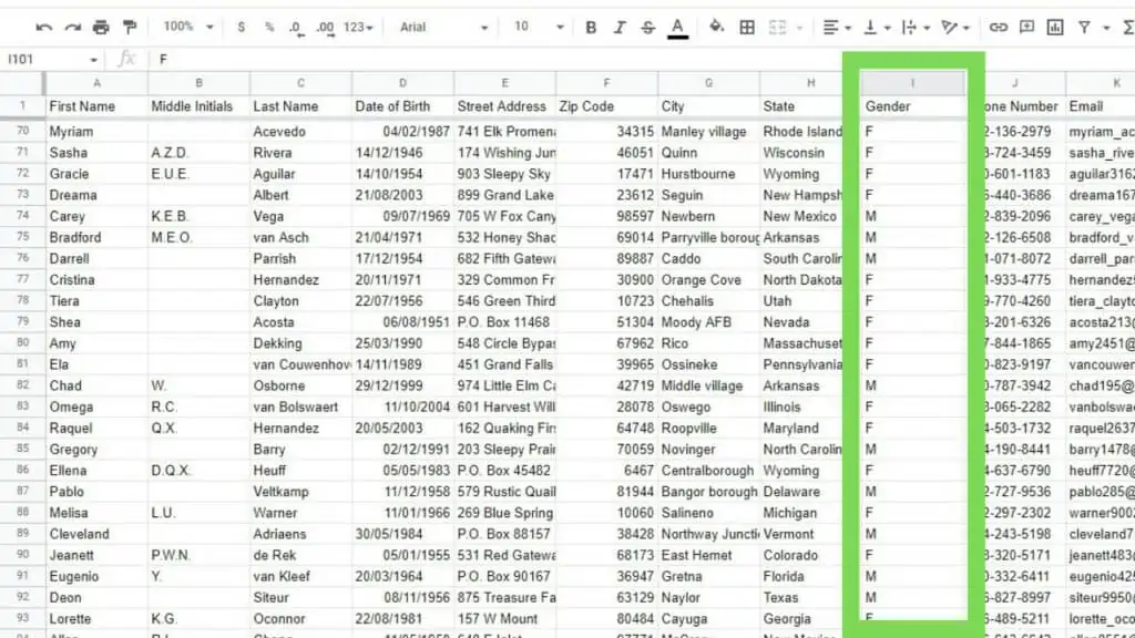
To start, we are identifying column I as the dataset for this example. The exact range is “I2:I101”. The criterion to count males is that if a cell in range I2:I101 is male, it should have ‘M’ which is an indicator that the record pertains to a male employee.

The formula for that will be “=COUNTIF(I2:I101,”M”)”.

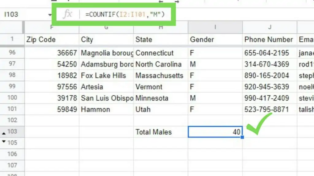
And with that, we get the count of male employees in the company to be 40.

To count the females, we just need to change the criterion from “M” to “F”.

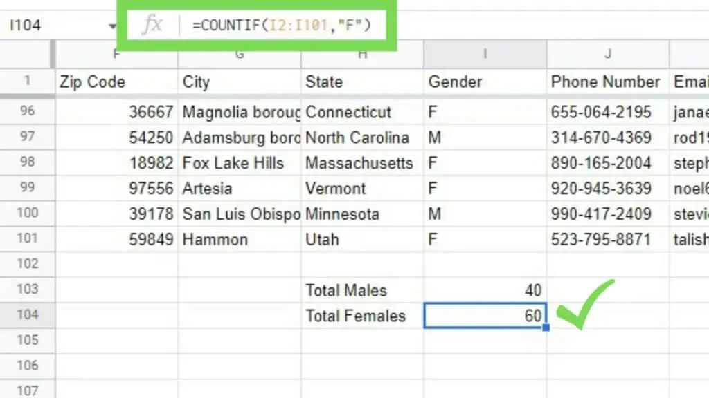
And with that, we can start making sound decisions to fund sex or gender-specific allocations using COUNTIF in Google Sheets.

With an Operator Criterion

We don’t always look for a defined set of things, sometimes we just want to know how many scored this much in a certain record. And we can certainly do that as well with COUNTIF in Google Sheets.

In the sample dataset below, I have a dataset of students with their scores recorded for a test.

I wanted to see how many students passed the required score of “80”. The formula for this is as follows: “=COUNTIF(E2:E101,”>=80″)”.

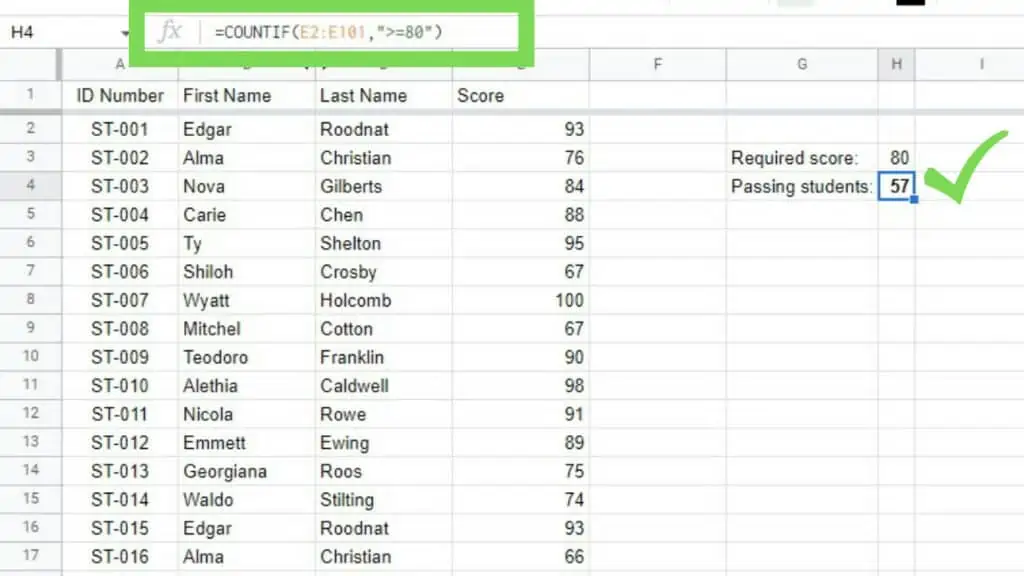
With this, I was able to identify how many of the students in this record passed the test.

With Multiple Criteria

There will be occasions when you’ll need COUNTIF in Google Sheets but you need to use it for more complex situations. Since this function only accepts one criterion, you are limited to simple expressions. For those cases, you can use the function COUNTIFS instead.

The COUNTIFS Function checks multiple ranges with each having its own criteria at the same time. Take note that for a certain value to be counted, it has to pass all criteria.

The syntax for COUNTIFS:

=COUNTIFS(criteria_range1, criterion1, [criteria_range2, criterion2, …])

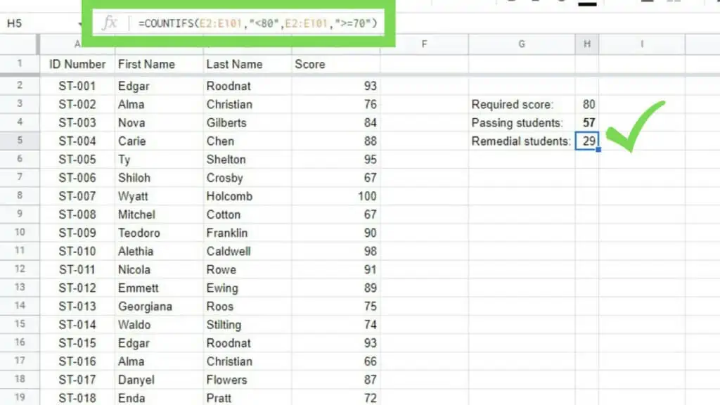
Following through with the last sample dataset, I wanted to count the number of students who have not reached the required score to pass but did not necessarily flunk out. Those with scores lower than “80” but higher than “70” will be given a remedial exam.

The formula for this specific condition is: “=COUNTIFS(E2:E101,”<80″,E2:E101,”>=70″)”.

There are alternative methods to inputting multiple criteria for COUNTIF in Google Sheets without using the COUNTIFS Function but they are more complex and oftentimes, unnecessary.

Using COUNTIFS is more versatile and you can even check multiple columns at the same time but they will be counted on a per-row basis only where each row passes all criteria checks defined in the ‘criteria’ parameter.

Frequently Asked Questions about How to Use COUNTIF in Google Sheets

Conclusion on How to Use COUNTIF in Google Sheets

To use COUNTIF in Google Sheets, identify the range that you want to apply COUNTIF to and then define the criterion that you want the dataset to be checked against. Use this formula: “=COUNTIF(range, criterion)”.