Do you want to see all the students with passing grades in a huge scoring dataset?
Or perhaps you have an inventory spreadsheet and you want to check if you still have everything in stock or maybe you need to reorder some items for restocking?
There are several ways you can solve such scenarios in Google Sheets.
Some resort to using Dot Plots in Google Sheets. But one easy way to make it visually appealing is through Conditional Formatting.
I’ll share how to take advantage of copying conditional formatting in Google Sheets so you can use it for multiple cells.
How to Copy Conditional Formatting in Google Sheets
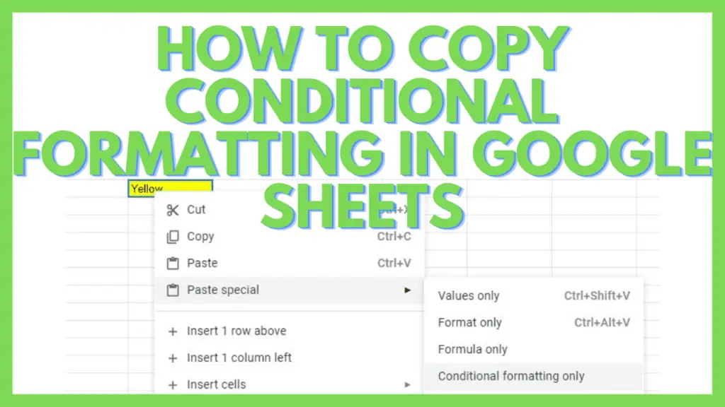
The easiest technique to copy conditional formatting in Google Sheets is the Copy and Paste Special Method:
- Right-click on the cell with the conditional formatting and click ‘Copy’
- Go to the destination cell and do a right-click
- Go to ‘Paste special’ and select ‘Conditional formatting only’

Copy Conditional Formatting in Google Sheets Video Tutorial
3 Effortless Techniques to Copy Conditional Formatting in Google Sheets
It’s simple to set up conditional formatting but it’s definitely easier to copy it once you have it all done at the start.
To know more about setting it up at first, read more about it in one of my other tutorials, How to Set Up Conditional Formatting.
Now, with the first technique, I just need to use Copy > Paste Special > Conditional formatting only.
For the second one, it will just need me to do a few clicks with the Paint format tool.
And for the last technique, I just need to get to the Conditional format rules pane and edit the range there.
Technique 1 to Copy Conditional Formatting in Google Sheets by using Copy > Paste Special > Conditional formatting only
Step one – I’ll select the source cell (where the conditional formatting will be copied from) and either hit Ctrl+C or do a right-click and select Copy.

Step two – I’ll go to the destination cell (where the conditional formatting that was copied will be pasted) and select it.
I will then do a right-click for the context menu to show up, hover the mouse icon over Paste special, and select Conditional formatting only.

And that’s one down.

We now see under Conditional format rules that E12 is now included in the range but it’s not reflecting the format because it hasn’t satisfied the condition yet.
To test if it’s really working, we just need to make the cell “not empty” so that it will satisfy the condition and apply the format on the cell causing the cell to have a yellow background.

By typing 1 (or any other character will do), the cell is no longer empty and is now reflecting the conditional formatting.
Consequently, emptying the cell will automatically change it back to its original background color.
Technique 2 to Copy Conditional Formatting in Google Sheets using the Paint format tool
Step one – I just need to select the source cell and then press the Paint format tool icon (located beside the Print icon by default).
This will copy and save the conditional formatting of the source cell.

Step two – Next, I will just need to select the destination cell. This will already apply the copied conditional formatting from the source cell to the destination cell.

The range in the Conditional format rule is now updated to include cell E5.
To check, we just need to satisfy the condition.

By typing 2 (or any other character will do), the cell is no longer empty and is now reflecting the conditional formatting.
Consequently, emptying the cell will automatically change it back to its original background color which is white.
Technique 3 to Copy Conditional Formatting in Google Sheets by using Format > Conditional Formatting > Edit “Apply to range”
Step one – I will select the source cell and go to the Menu bar, press Format, and select Conditional formatting.

This will cause the Conditional format rules pane to show up displaying the rules that you have that affect your selected cell or range.

Step two – Select the rule that you want to copy. Then update the range to include the cell (or cells) that you wish to have the same conditional formatting applied. Press Done once you’re finished.

This should now copy the conditional formatting from cell D5 to cell E5. To test it out, I just need to satisfy the condition and make cell E5 not empty.

By typing 3 (or any other character will do), the cell is no longer empty and is now reflecting the conditional formatting. Consequently, emptying the cell will automatically change it back to its initial background color.
As you can see, I was only able to put in two steps for each of the three techniques as it really is just that simple to copy conditional formatting in Google Sheets.
This time, it really just depends on your preference but there may be times when one method is a little bit easier to use than the rest.
For example, if you’re applying conditional formatting to a huge range of cells, it may be best to use Technique 3 as you can just type in the range and you’re done.
Another example will be if you are copying single conditional formatting to multiple single separate cells, I would advise that you use Technique 2. As it will be so much easier with the Paint format tool.
And for everything else, I would suggest you use Technique 1 as depending on the situation, it may be easier to use than the other two. Plus, it’s quite easy to access with just a right-click of your mouse.
Frequently Asked Questions About How to Copy Conditional Formatting in Google Sheets
How do I find the rules that I’ve just set up in Google Sheets if I can’t remember where it is?
You need to select all cells by clicking on the box above Row 1’s box and by the left side of Colum A’s box. This will cause all cells to be selected. Then go to the Conditional format rules window to see them.
Can I copy Conditional Formatting rules to a different sheet in Google Sheets?
You cannot copy conditional formatting rules to a sheet in a different Google Spreadsheet. Instead, you can make a copy of it on the destination workbook. Then use Copy > Paste Special > Conditional formatting.
Conclusion About How to Copy Conditional Formatting in Google Sheets
To copy conditional formatting in Google Sheets, right-click on the cell with the conditional formatting and click ‘Copy’. Then go to the destination cell to do a right-click. Finally, go to ‘Paste special’ and select ‘Conditional formatting only’.

