Check if a Row Contains a Number or Text in Google Sheets

It gets tricky when you’re trying to figure out if a cell or row contains a specific letter or number that you’re looking out for if you’re just using the search function via CTRL+F or an IF-contains formula in Google Sheets.

Both can still be usable if you have a small dataset, but what if you have multiple rows? There must be a better way to check if a row contains a number or text in Google Sheets.

True enough, there are various functions that will let you know if a row contains a number or text in a much simpler way.

And that is why in this tutorial I am going to show you how to check if a row contains a number or text in Google Sheets.

How to Check if a Row Contains a Number or Text in Google Sheets

1. Define the row that you wish to check for a number or text (for example, 1:1 or 2:2)
2. Decide if you want to check for a number, text, or a combination of both.
3. Use the appropriate REGEXMATCH formula depending on what you’re looking for.
4. If the row that you’re checking contains what you’re looking for, you will get the output: ‘TRUE’.

Using REGEXMATCH to Check if a Row Contains a Number or Text in Google Sheets

We use REGEXMATCH to check strings if they contain a specific substring or character.

This is how we can check if a row contains a number or text in Google Sheets.

Depending on what you’re looking for, a different formula is suited specifically.

Below are some examples of specific scenarios.

Take note that the “row_reference” part of the formulas pertains to the range parameter of the JOIN function (for example, 1:1 or 2:2).

How to Check if a Row Contains Lower-Case Characters Only

To check for lower-case characters only, use the formula below:

=REGEXMATCH(JOIN(“”,row_reference),”[a-z]”)

The JOIN function is added to be part of the cell_reference parameter of the REGEXMATCH function. This is to make sure that everything in the row being checked is included.

The “[a-z]” regular expression which makes the 2nd parameter of the REGEXMATCH function refers to all lower case letters from ‘a’ to ‘z’.

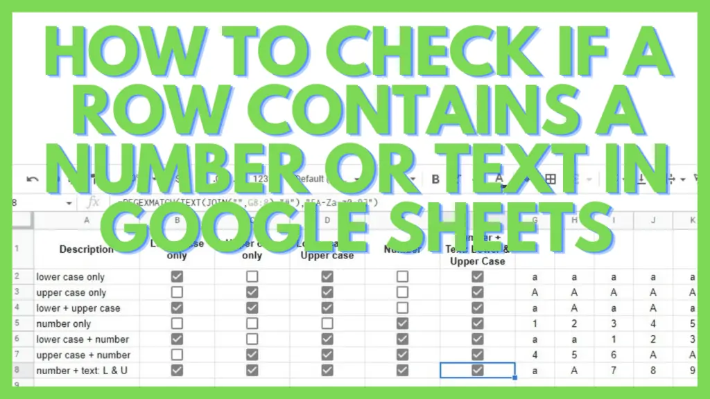
As seen in the example with varying characters in the range G2:K8, only the rows containing at least 1 lowercase ‘a’ have a checkmark in the first column (equivalent to ‘TRUE’).

This formula will return a ‘FALSE’ for characters such as upper-case letters, numbers, and symbols.

Check if a Row Contains Upper-Case Characters Only in Google Sheets

To check for upper-case characters only, use the formula below:

=REGEXMATCH(JOIN(“”,row_reference),”[A-Z]“)

The “[A-Z]” regular expression which makes the 2nd parameter of the REGEXMATCH function in this case refers to all upper case letters from ‘A’ to ‘Z’.

As seen in the example with varying characters in the range G2:K8, only the rows containing at least 1 upper case ‘A’ have a checkmark in the first column (equivalent to ‘TRUE’).

This formula will return a ‘FALSE’ for characters such as lower-case letters, numbers, and symbols.

Check if a Row Contains Both Lower-Case and Upper-Case Characters 

To check for either or both lower-case and upper-case characters, use the formula below:

=REGEXMATCH(JOIN(“”,row_reference),”[a-zA-Z]”)

The “[a-zA-Z]” regular expression makes the 2nd parameter of the REGEXMATCH function, in this case, refer to all lower case letters from ‘a’ to ‘z’ and upper case letters from ‘A’ to ‘Z’.

As seen in the example with varying characters in the range G2:K8, only the rows containing at least 1 lower case ‘a’ OR an upper case ‘A’ have a checkmark in the first column (equivalent to ‘TRUE’).

This formula will return a ‘FALSE’ for characters such as numbers and symbols.

How to Check if a Row Contains Numbers Only in Google Sheets

To check for numbers only, use the formula below:

=REGEXMATCH(TEXT(JOIN(“”,row_reference),”#”),”[0-9]”)

Aside from changing the regular expression to “[0-9]” which denotes any number from 0 to 9, we also added the TEXT function.

The REGEXMATCH function in Google Sheets only accepts text as its first parameter so cells containing numbers only will be skipped.

With the TEXT function, they’ll be converted to text and thus be accepted by the REGEXMATCH function.

The “[0-9]” regular expression makes the 2nd parameter of the REGEXMATCH function, in this case, refer to all numbers from ‘0’ to ‘9’.

As seen in the example with varying characters in the range G2:K8, only the rows containing at least 1 number have a checkmark in the first column (equivalent to ‘TRUE’).

This formula will return a ‘FALSE’ for characters such as letters and symbols.

Check if a Row Contains Numbers, Lower-Case, or Upper-Case Characters

To check for lower-case or upper-case characters, numbers, or any combination of letters and numbers in Google Sheets, use the formula below:

=REGEXMATCH(TEXT(JOIN(“”,row_reference),”#”),”[A-Za-z0-9]”)

Similar to the previous formula which looks for numbers, this one also includes the TEXT function.

The “[A-Za-z0-9]” regular expression makes the 2nd parameter of the REGEXMATCH function, in this case, refer to all lower case letters from ‘a’ to ‘z’, upper case letters from ‘A’ to ‘Z’, and numbers from ‘0’ to ‘9’.

As seen in the example with varying characters in the range G2:K8, only the rows containing at least 1 number or a letter have a checkmark in the first column (equivalent to ‘TRUE’).

This formula will return a ‘FALSE’ for characters such as symbols.

“=REGEXMATCH(TEXT(JOIN(“”,row_reference),”#”),”[A-Za-z0-9]”)” is the best formula to check if a row contains a number or text in Google Sheets.

Frequently Asked Questions about How to Check if a Row Contains a Number or Text in Google Sheets

Conclusion on How to Check if a Row Contains a Number or Text in Google Sheets

To check if a row contains a number or text in Google Sheets, select the row to be checked, and decide if you’re looking for a number or text. Use the REGEXMATCH formula matching your needs. The formula “=REGEXMATCH(TEXT(JOIN(“”,row_reference),”#”),”[A-Za-z0-9]”)” will allow you to check if a row contains a number or text in Google Sheets.