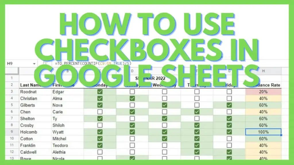
In this tutorial, I will show you how to use checkboxes in Google Sheets.
Anyone working in a corporate or government office will more than often encounter tick boxes in the way of forms and checklists. It just shows how important it is to indicate that something is applicable or true.
Tick boxes or checkboxes in Google Sheets are a feature that I often use instead of displaying TRUE or FALSE.
How to Use Checkboxes in Google Sheets
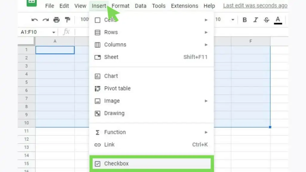
- Select a cell or range where you want the checkboxes to be
- Go to the Insert menu
- Select Checkbox
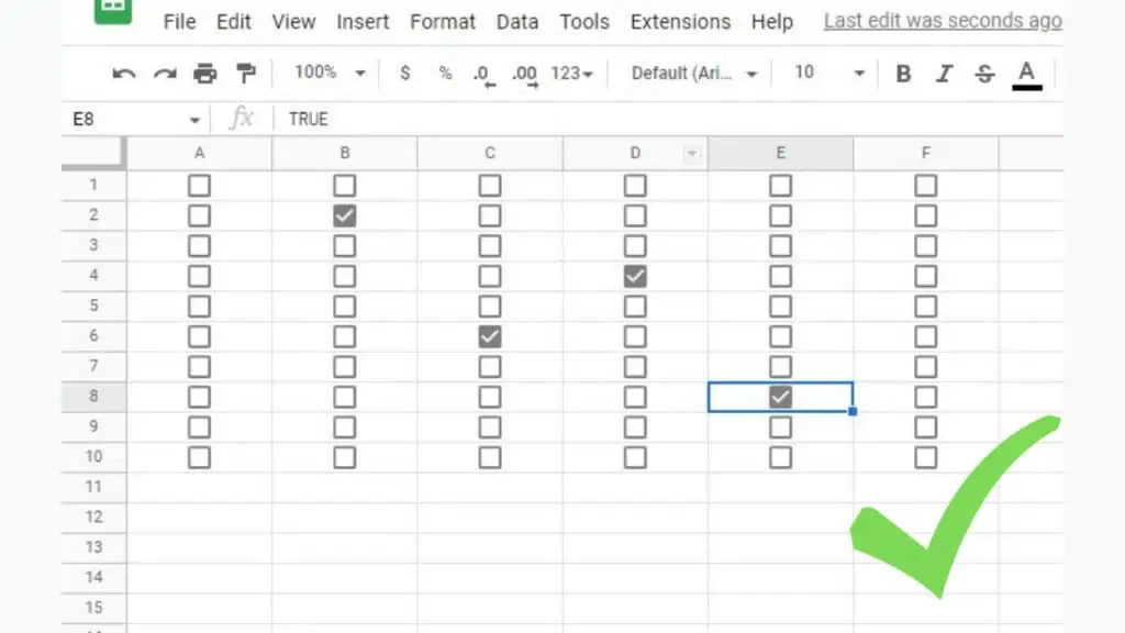
- Click on a checkbox to put a checkmark on it

Use Checkboxes and Checklists in Google Sheets Video Tutorial
Inserting Checkboxes in Google Sheets
Checkboxes in Google Sheets are an interactive feature in Google Sheets where you can display an empty box or a box with a check mark.
This is different from a check mark ✔ in that a check box may or may not have a checkmark and is functional while the former is a special character.
To insert a checkbox, start by selecting a cell or a range and then going to the ‘Insert’ menu. Once there, click on ‘Checkbox’.
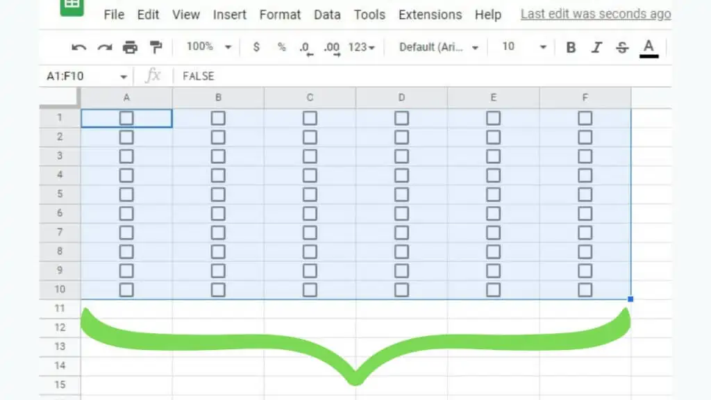
This should instantly add empty checkboxes to every cell selected.
An empty checkbox has a value of FALSE. While a ticked checkbox has a value of TRUE.
Clicking on any checkbox will switch its equivalent value from FALSE to TRUE and vice-versa.
You can also copy a cell with a checkbox and paste it on another cell to duplicate a checkbox without going through the menu.
Checkbox Example in Google Sheets
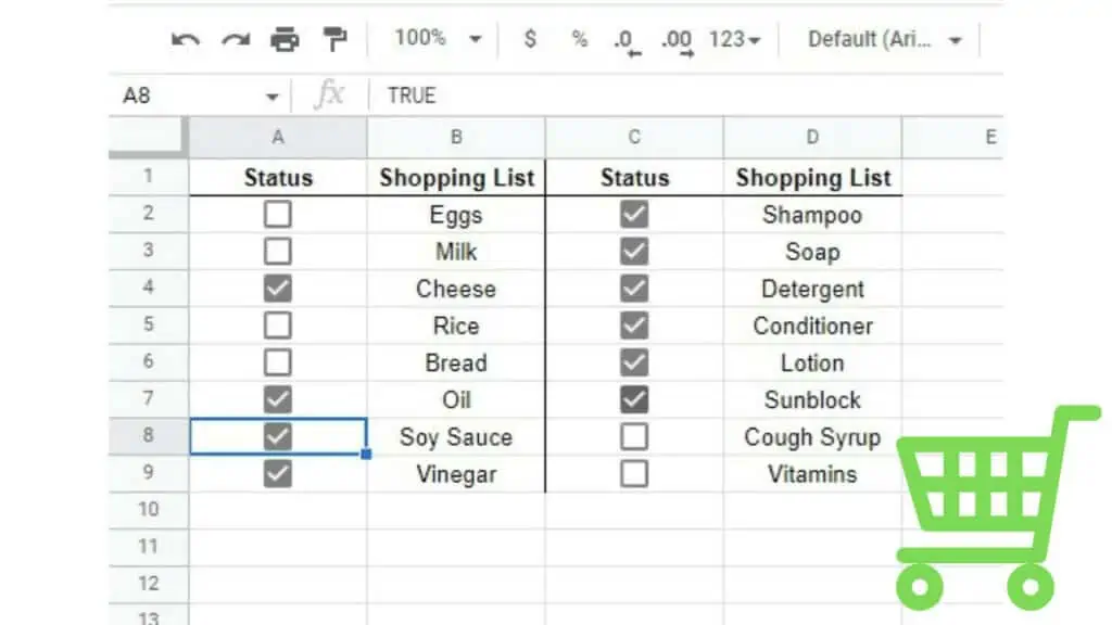
Checkboxes in Google Sheets can be really simple in that oftentimes, they are only used as a visual representation of “checked items” such as tasks completed, items ordered, etc.
The example below is a simple shopping list.
Once I acquire a certain item, I just have to click on the associated checkbox and that indicates that I’m done with that item and that I have purchased it.
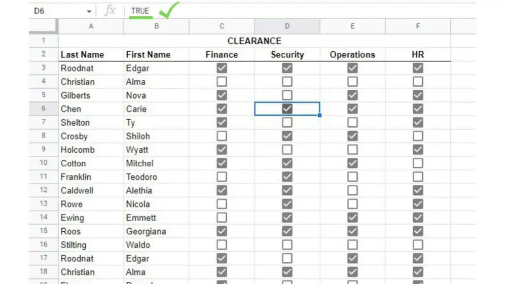
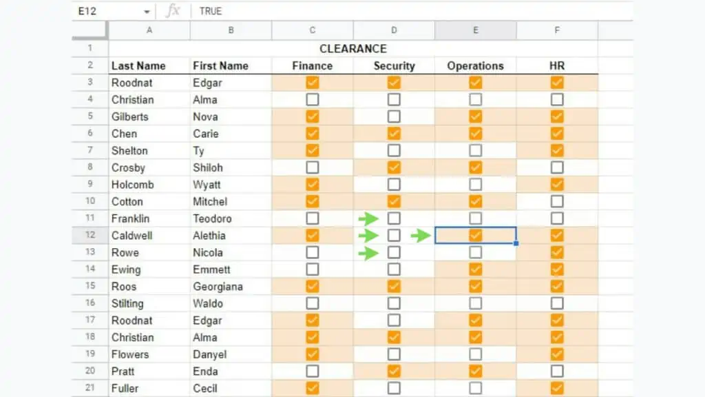
It can be a bit more complex like in the example below where there are 20 names under the clearance record file where their clearance status with different departments is indicated.
This can be considered a master file and can also act as a backup system. That means that in cases where something happens to other records, this table with checkboxes can be used to recover data.
Same with the above, anyone with edit access to a spreadsheet can simply click on a checkbox to change it from FALSE to TRUE and vice-versa.
If you have a table with binary results such as 0 or 1, TRUE or FALSE, and others, you may use the checkbox to store such data. As for 0 or 1, you need to convert them to TRUE or FALSE first.
Normally, 0 is associated with FALSE while 1 is TRUE.
In the example below, I have a table that is pre-filled with TRUE and FALSE values.
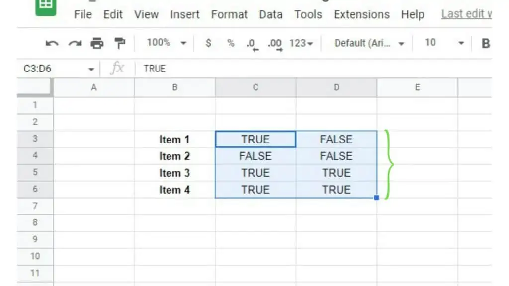
I only need to select the cells containing the TRUE or FALSE values and then go to ‘Insert’ and select ‘Checkbox’.
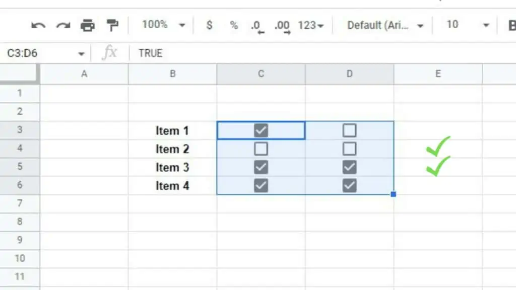
This will instantly insert checkboxes that will be automatically ticked if the value prior to inserting a checkbox is TRUE.
Formatting Checkboxes in Google Sheets
Since checkboxes in Google Sheets are mostly treated as visual aids, it helps to know that a checkbox can also be applied with formatting tools such as coloring, alignments, and size since they are treated the same as regular text.
In the example below, I demonstrated how checkboxes can be colored as well.
To start, I simply selected the cells containing the checkboxes to be formatted.
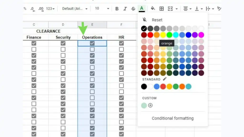
Next, I simply have to use the applicable formatting tools. In this example, I selected Text Color and picked ‘Orange’.
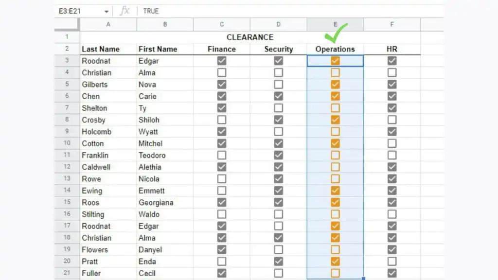
This immediately changes the color of the checkboxes that I have selected to the color that I picked.
Conditional Formatting for Checkboxes in Google Sheets
In the same way that checkboxes can be formatted like text, it’s also a great idea to apply ‘Conditional formatting’ to them. You can apply a certain set of formatting to a specific subset within the range that you’ve selected based on certain criteria.
For example, you can change the color of checkboxes in Google Sheets that are ticked. Another great thing about this is that if you untick a checkbox, the formatting will disappear since it no longer satisfies the conditions of conditional formatting.
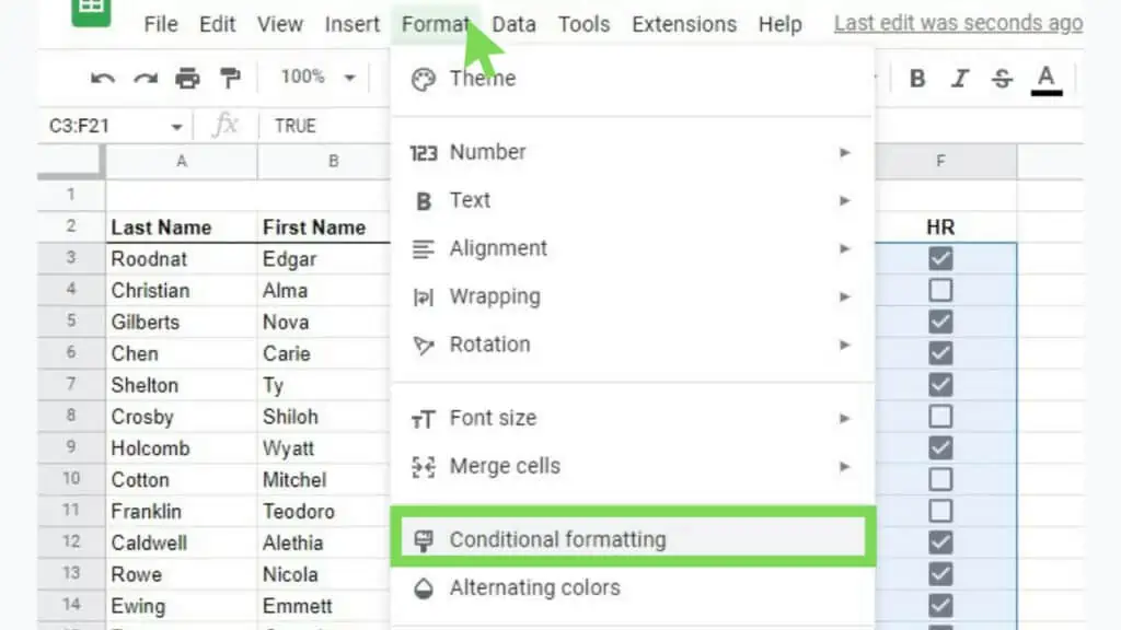
To do this, just select the cells containing the checkboxes that you would like to be applied with conditional formatting.
Next, go to ‘Format’ and select ‘Conditional formatting’.
In the ‘Conditional format rules’ window, the range should be okay now if you select them properly, but if you need to, you may edit and change it at this point.
For the ‘Format rules’, select IS EQUAL TO and set the value to TRUE.
This means that if, and only if, a checkbox contains TRUE (therefore is ticked), the following ‘Formatting style’ will be applied.
You may change the ‘Formatting style’ to your preference. Once you’re satisfied, hit DONE.

This should now change all selected checkboxes in Google Sheets to the prescribed formatting style. To confirm if the conditional formatting works, I’ll toggle checkboxes in D11:D13 as well as E12.
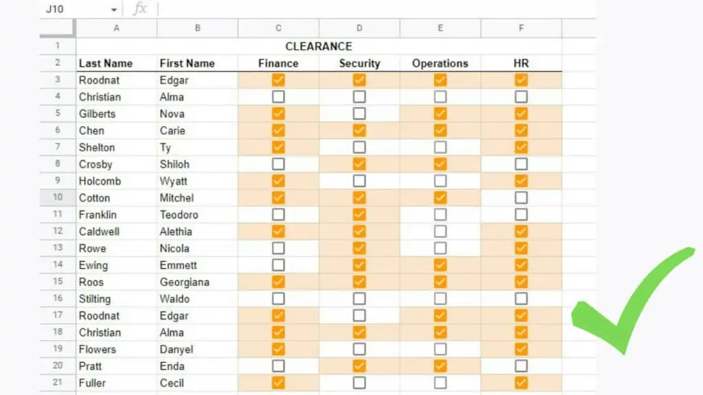
As you can see below, aside from the checkmark presence, the formatting style has also been removed and applied respectively.
As checkboxes in Google Sheets are often used for their helpful visual properties, conditional formatting can help in boosting its potency to deliver information.
Create Dynamic Charts with Checkboxes in Google Sheets
Finally, other than checkboxes in Google Sheets, the top-tier visual representation is charts.
And one last great thing that I would like to show you about checkboxes is how they can be used to “toggle” chart data as well.
This manipulation can be done due to the fact that blank cells, rows, or columns are not represented in graphs.
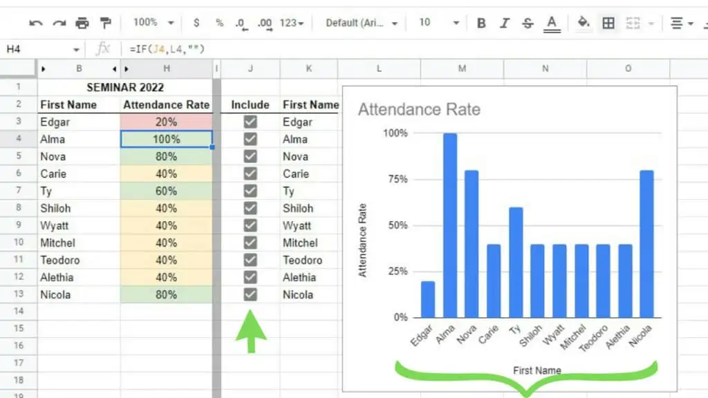
In the example below, other than the main data table where the names and attendance rates are put in, I created a toggle checklist in the Include column along with each First name for the association.
Take note of the chart and how it appears as the table still has all its contents.
In the next example, I “toggled off” the records for Nova, Mitchel, and Alethia. In effect, their respective rows became blank and the chart was instantly updated to show the remaining information only.
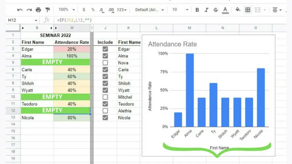
This can be done by editing the main table and adding an IF Function where if the Include toggle is ticked, the data is visible and will appear as blank if otherwise.
The IF syntax used in the table for this purpose is:
=IF(toggle_cell_reference, table_cell_contents, “”
Where
- toggle_cell_reference is the checkbox to determine if a value is to be included (column J in the example)
- table_cell_contents is the value output for the table or main dataset
- “” is the value_if_false parameter of the IF Function where “” indicates blank
This is a great way to not only make charts more focused depending on how you set it.
Checkboxes in Google Sheets are so useful from their visual capabilities up until their toggle function allowing us to modify formulas and even graphs that were already set up. I recommend to anyone using Google Sheets to master and take advantage of checkboxes as soon as they can.
Frequently Asked Questions about How to Use Checkboxes in Google Sheets
How can I insert checkboxes in Google Sheets?
To insert checkboxes in Google Sheets, select the cells where you want the checkboxes to be, then go to the ‘Insert’ menu, and select the ‘Checkbox’ option. Alternatively, if you have existing checkboxes, you may also copy and paste them to a different cell.
How can I use checkboxes in Google Sheets?
To use checkboxes in Google Sheets, simply click on them to toggle them from unticked to ticked and vice-versa. You may also manually type in TRUE (ticked) or FALSE (unticked) in the formula bar once you click a cell with a checkbox.
Conclusion on How to Use Checkboxes in Google Sheets
You can use checkboxes in Google Sheets by first selecting a cell or range where you want the checkboxes to be. Next, go to the Insert menu and select the Checkbox option. You may now click on a checkbox to put a checkmark in it.

