Are you currently handling large amounts of data that you are looking to summarize so you can get some relevant insights? A tool that you can utilize for this is the pivot table.
A Pivot Table gives you the capability to group and simplify huge sets of data and lets you utilize an assorted range of summarizing metrics to assist you in your data analysis.
Moreover, the Pivot Table comes with the ‘Calculated Field’ feature which allows you to customize the Pivot table results with formulas and functions.
In this tutorial, I am going to show you how to add and use a calculated field in Google Sheets.
How to Add and Use a Calculated Field in Google Sheets
To add and use a calculated field in Google Sheets:
- Prepare your pivot table and go to the ‘Pivot table editor’
- Click the ‘Add’ button on the right side of Values’
- Select ‘Calculated field’ from the dropdown menu that appears
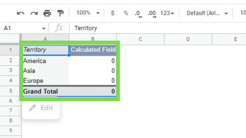
- A new ‘Calculated Field’ column will be added to your table.
- Go to the ‘Calculated Field 1’ window in the ‘Pivot table editor’
- Update the ‘Calculated Field’ properties accordingly

Preparing the Pivot Table
Before you can add a calculated field in Google Sheets, the pivot table where it is to be added needs to be prepared.
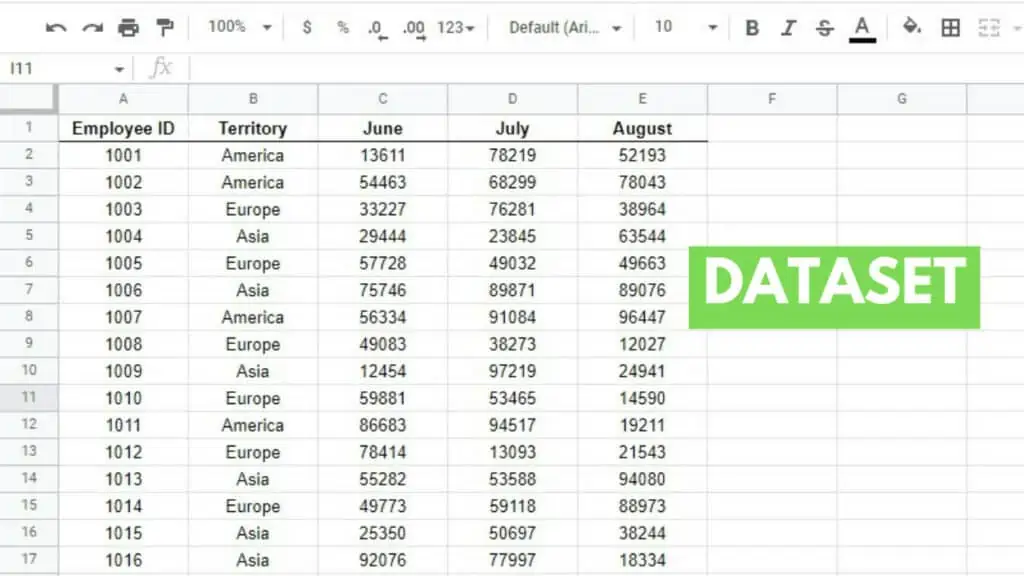
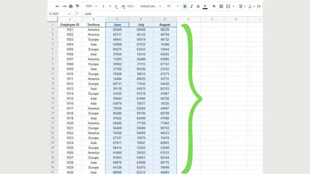
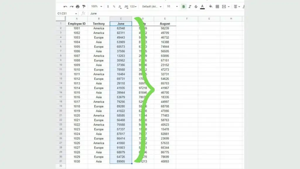
Below is a sample dataset of employees’ sales across three months in 3 continental territories. We’re going to use a pivot table and calculated fields to summarize some points that we’ll be identifying later in this tutorial.
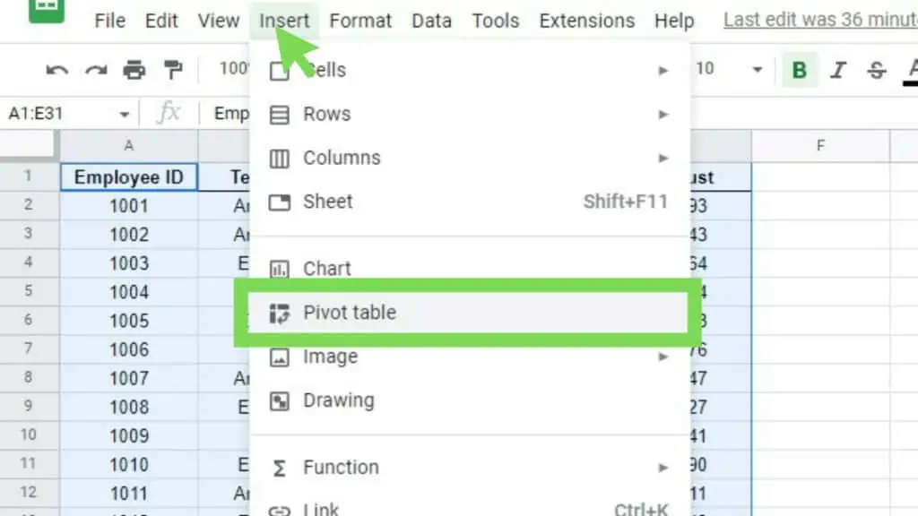
Select the data range and go to the ‘Insert’ menu, and select ‘Pivot table’.
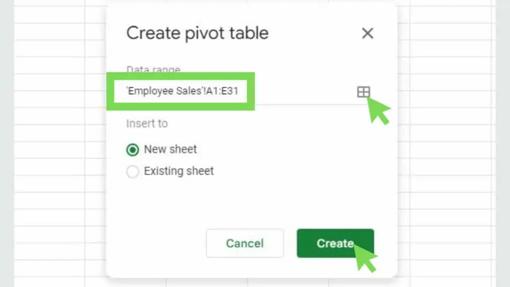
The ‘Create pivot table’ will appear. If you have selected the data range properly, it will appear in this window. If you need to edit the range, just click on the icon on the left side of the ‘Data range’ field.
You may select ‘New sheet’ for the ‘Insert to’ option where the pivot table will automatically be placed into a new sheet.
Alternatively, choosing ‘Existing sheet’ will prompt you to input the exact cell address where you want the pivot table to be.
Once you’re good with the options for the pivot table, hit ‘Create’.
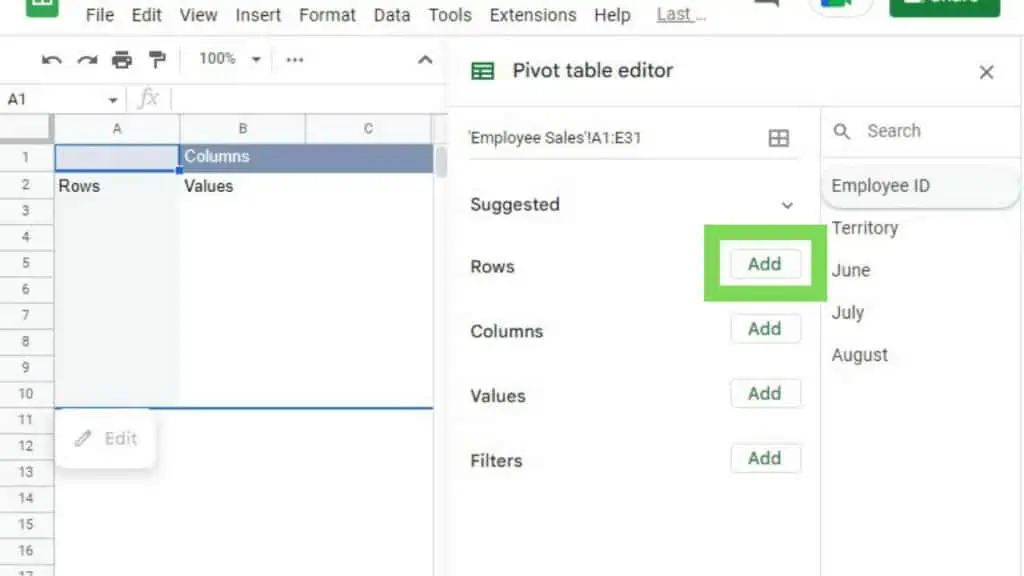
On the sheet where the pivot table is, the ‘Pivot table editor’ will appear. If you close it, you can reopen it by clicking the ‘Edit’ button below the pivot table.
Click on the ‘Add’ button on the right side of ‘Rows’.
For this example, we’re going to select ‘Territory’.
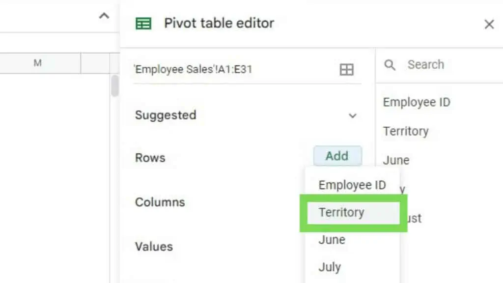
As soon as it’s selected, the Territory unique values in our dataset will appear as rows of the pivot table.
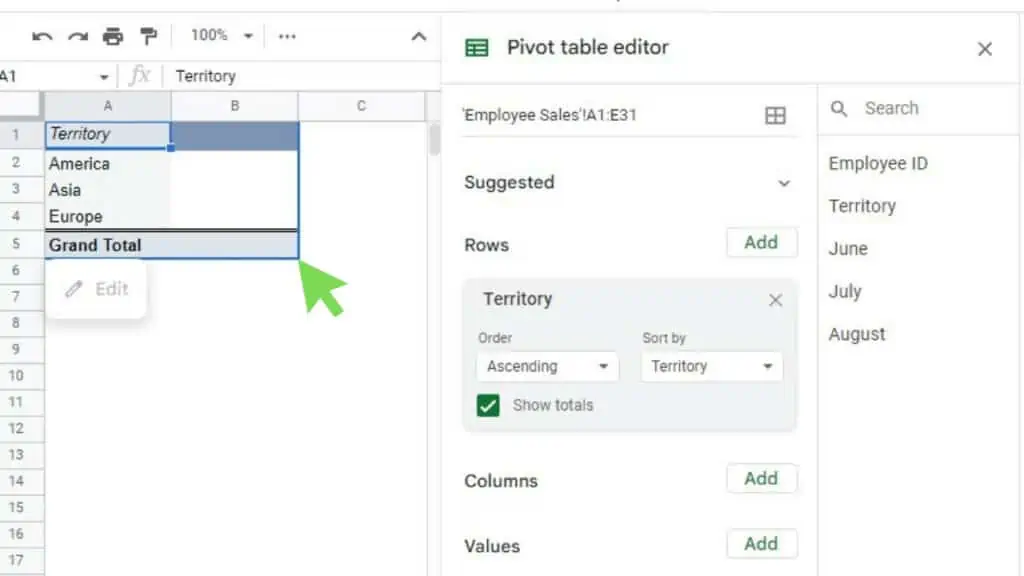
We now have a basic pivot table for our sample dataset. We’re now going to input a calculated field in Google Sheets.
Adding the Calculated Field
A calculated field in Google Sheets is a feature of the Pivot table. It contains a special formula that refers to other fields of the original dataset.
To add the calculated field, we’ll start by clicking on the ‘Add’ button on the right side of ‘Values’.
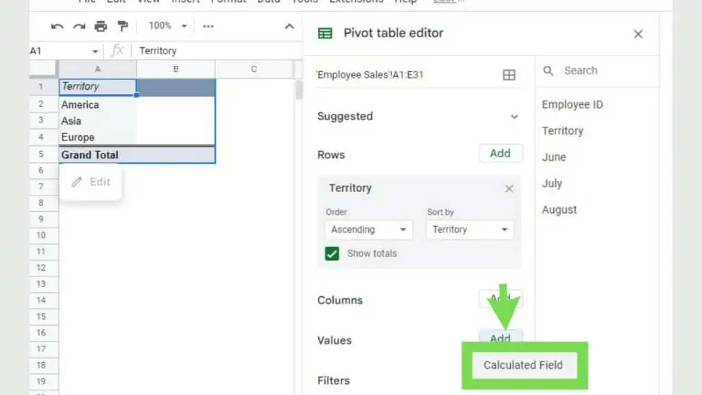
This will add a ‘Calculated Field’ column to the Pivot table which will have 0 values until we set it up.
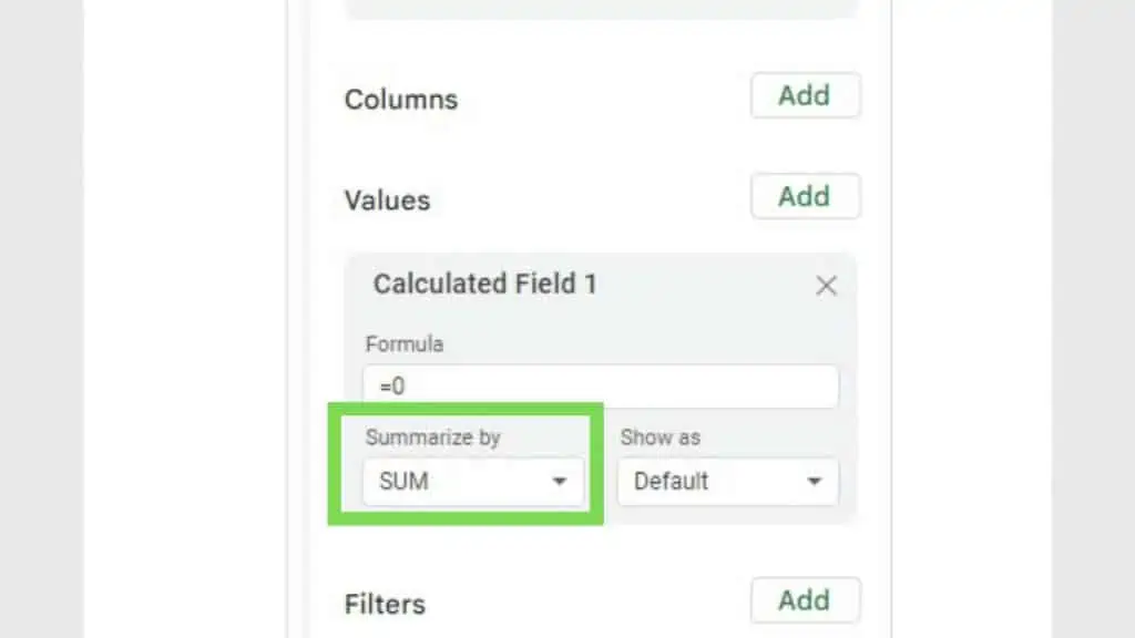
On the ‘Pivot table editor’, we’re going to update the formula so that it’ll reflect the values that we want. By default, it is summarized by ‘SUM’ but this can be changed to ‘CUSTOM’ for any other formula requirement.
As mentioned, we’re going to be discussing two options to summarize a calculated field in Google Sheets.
Summarizing a Calculated Field by SUM
To summarize a calculated field in Google Sheets by sum, we just need to identify the parts of the datasets to be added.
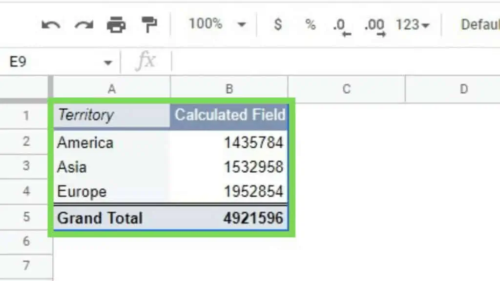
Use the exact names of the header or columns from the original dataset as part of the Formula as seen in the example below. Keep the ‘Summarize by’ field as ‘SUM’ and hit enter (if the pivot table values won’t update).
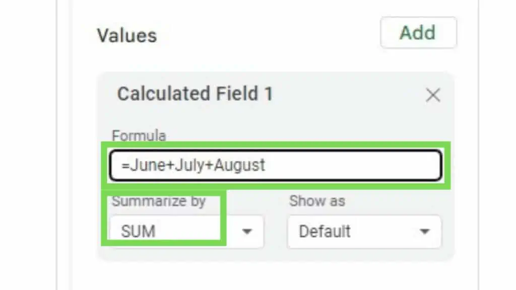
As you can see, the total amount of sales per territory from June to August in our dataset is computed and reflected in the ‘Calculated Field’.
Summarizing by Custom Formula
To summarize a calculated field in Google Sheets by using a custom formula, we need to identify the parts of the datasets to be added in their proper function format.
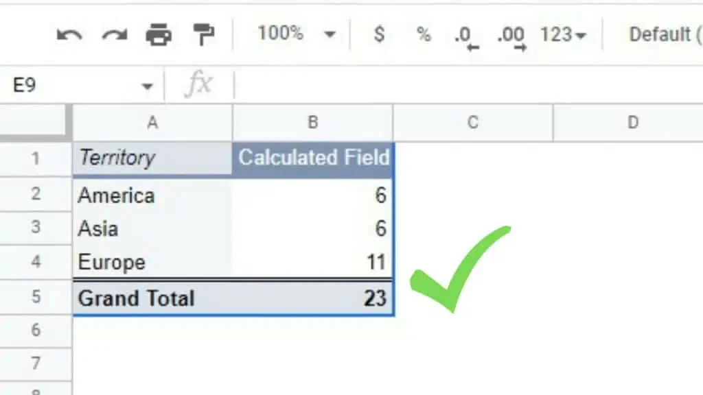
For this example, we’re going to be counting the number of employees who had sales of over 40000 per territory in June.
We can do this by typing in the following formula:
=COUNTIF(June,”>40000”)
As you can see, we used the header ‘June’ to identify the column where the data will be taken from.
We also need to change the ‘Summarize by’ value to ‘Custom’.
The pivot table has been updated to reflect the number of employees per territory in the month of June whose sales exceed 40000.
Pivot tables by themselves are really useful but utilizing a Calculated Field in Google Sheets or pivot table charts can bring your data presentation and analysis to the next level.
Frequently Asked Questions about How to Add and Use a Calculated Field in Google Sheets
How do I add and use a calculated field in Google Sheets?
Click the ‘Values’ Add-button in the Pivot table editor and select ‘Calculated field’ from the menu. In the field under ‘Formula’, enter your formula (use the correct column names from the original table). Lastly, pick the ‘SUM’ or ‘Custom’ option as needed from the dropdown menu under ‘Summarize by’.
How do you input a custom function in a Google Sheets calculated field?
After adding the calculated field, a description box in the Pivot table editor will appear. Enter your custom function in the field under ‘Formula’. Double-check if it uses the correct field names. Make sure to enclose spaces in single quotes.
Conclusion on How to Add and Use a Calculated Field in Google Sheets
To add and use a calculated field in Google Sheets, prepare your pivot table, go to the ‘Pivot table editor’, and click the ‘Add’ button by the right side of Values’. Select ‘Calculated field’ from the dropdown menu that appears and go to the ‘Calculated Field 1’ window in the ‘Pivot table editor’. Update the ‘Calculated Field’ properties accordingly

