In this tutorial, I will teach you how to add Week, Month, and Quarter categories to dates in Google Sheets.
Categorizing dates into their respective Week, Month, and Quarter categories in Google Sheets will help prepare your data for visualization.
You can then use these categories to view things such as weekly income, monthly profit, quarterly expenses, and more in Google Sheets.
This is especially useful for preparing enormous amounts of data to be processed by a Pivot Table, which you can then use for a Pivot Chart.
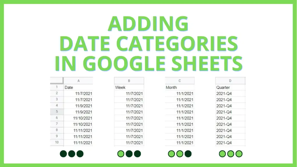
Adding Date Categories in Google Sheets
To Add Date Categories in Google Sheets:
- Add data to Google Sheets
- Add and adjust this formula to categorize a date to its week:
“=DATE(YEAR([date]),MONTH([date]),(DAY([date])-WEEKDAY([date])+[week start]))” - Add and adjust this formula to categorize a date to its month:
“=DATE(YEAR([date]),MONTH([date]),1)” - Add and adjust this formula to categorize a date to its quarter:
“=YEAR([date])&”-“&”Q”&ROUNDUP(MONTH([date])/3)” - Add and adjust the ARRAYFORMULA to categorize a date range into weeks, months, and quarters, respectively:
“=ARRAYFORMULA(IF([date range]=””,””,DATE(YEAR([date range]),MONTH([date range]),(DAY([date range])-WEEKDAY([date range])+1))))”
“=ARRAYFORMULA(IF([date range]=””,””,DATE(YEAR([date range]),MONTH([date range]),1)))”
“=ARRAYFORMULA(IF([date range]=””,””,YEAR([date range])&”-“&”Q”&ROUNDUP(MONTH([date range])/3)))”
How to Add Date Categories in Google Sheets
For this tutorial, I have prepared a dummy dataset containing a random succession of dates.
Additionally, I have expanded the dummy dataset to contain a relatively large amount of dates.
Feel free to apply these steps and formulas to any number of rows that you are comfortable with, or to even apply it to categorize your own set of dates.
Step 1 – Add data to Google Sheets
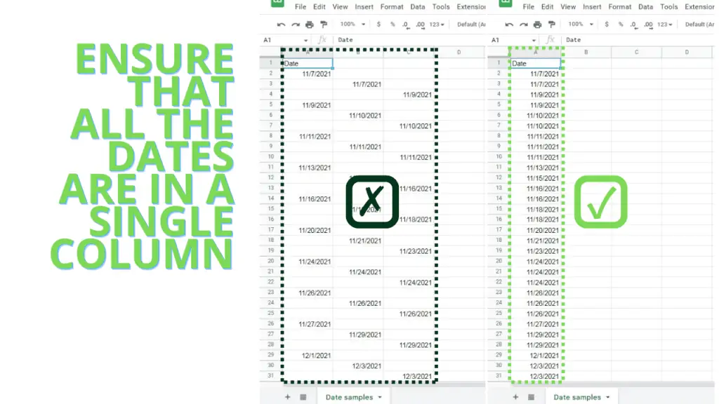
First, we will need to have dates to apply our formulas on. For that, you can use any set of dates that you have, or you can use the dataset that I have mentioned through this link.
If you opt to use your own data, I advise that you place them in a single column as this will simplify the application of the same formulas across multiple rows.
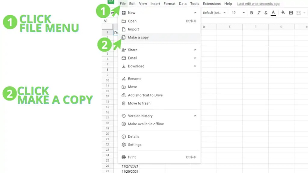
For the dataset that I’ve provided, you can make a copy of it by clicking ‘Make a Copy’ under the ‘File’ tab.
Step 2 – Add a formula to categorize a date to its week
Our next step involves adding a formula that transforms a date into a weekly date grouping.
On the column to the right of your chosen date, add the formula:
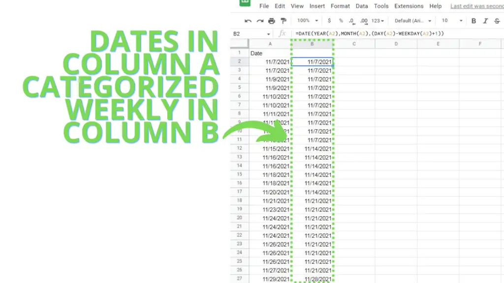
=DATE(YEAR([date]),MONTH([date]),(DAY([date])-WEEKDAY([date])+[week start]))
With the above formula, simply substitute the [date] parts with the address of the cell that your chosen date is in.
Next, substitute [week start] with a number that represents the day that your weekly groupings begin with: 1 for Sundays, 2 for Mondays, 3 for Tuesdays, etc.
Finally, copy the formula for all the rows in the same column.
As an example on the data that I provided, to categorize the date in A2 into weekly groupings that start on Sundays, the formula and result should look like this:
Step 3 – Add a formula to categorize a date by its month
The next step will involve adding a formula that transforms a date into a monthly date grouping.
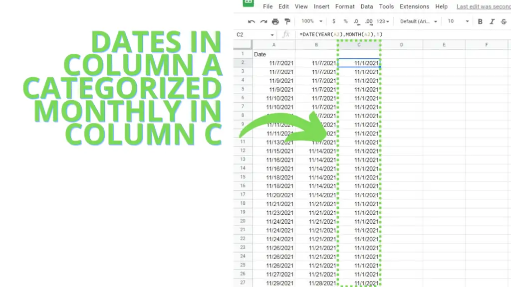
On the corresponding cell to the right of the cell where Step 1 was performed, add the formula:
=DATE(YEAR([date]),MONTH([date]),1)
On the above formula, simply substitute the [date] parts with the address of the cell that your chosen date is in.
Make sure that the referenced cell is the original date and not the cell where Step 1 was performed.
Finally, copy the formula for all the rows in the same column.
As an example on the data that I provided, to categorize A2 into monthly groupings, the formula and result should look like this:
Step 4 – Add a formula to categorize a date to its quarter
The next step will involve adding a formula that transforms a date into a quarterly date grouping.
On the corresponding cell to the right of the cell where Step 2 was performed, add the formula:
=YEAR([date])&”-“&”Q”&ROUNDUP(MONTH([date])/3)
On the above formula, simply substitute the [date] parts with the address of the cell that your chosen date is in, similar to the previous steps.
As an example on the data that I provided, to categorize A2 into Quarterly groupings, the formula and result should look like this:
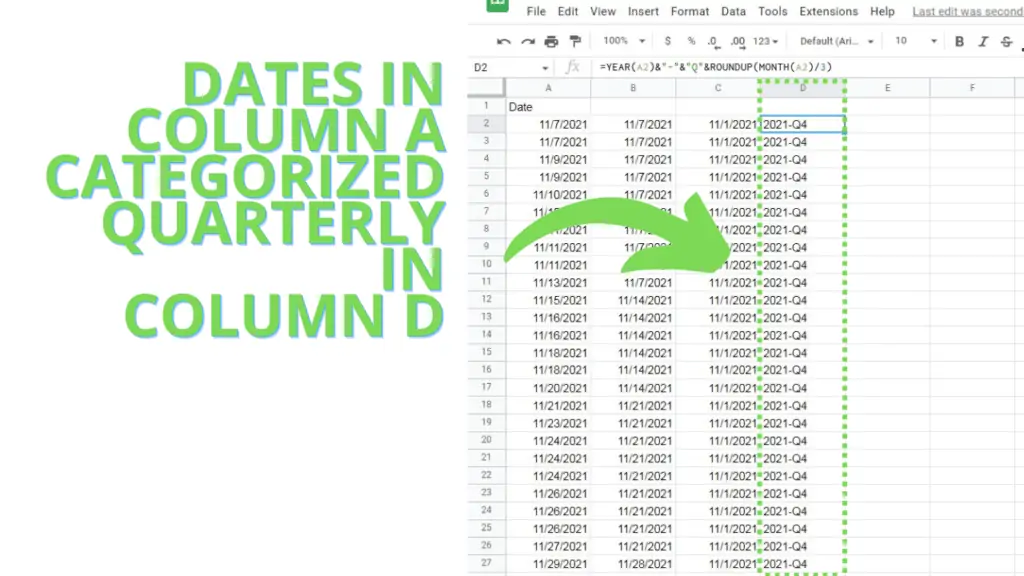
You may notice that the formula is not formatted to be a date, this is an optional formula whose result is easier to identify as a quarterly grouping.
To have a quarterly grouping in the format of a date, you can choose to use this formula structure instead:
=DATE(YEAR([date]),IF(MONTH([date])<=3,1,IF(MONTH([date])<=6,4,IF(MONTH([date])<=9,7,10))),1)
Similar to the previous formulas, substitute the [date] parts with the address of the cell that your chosen date is in.
Step 5 – [Advanced] ARRAYFORMULA usage
Finally, we move on to the application of the previous formulas with an ARRAYFORMULA.
This is an optional part, but you may find it useful in adding date categories to very large datasets that are continuously updated.
A very common application is in adding weekly, monthly, and quarterly categories on Google Forms responses within Google Sheets. As new forms are submitted, you would otherwise have to apply the formulas in steps 1, 2, and 3 to each new row.
With an ARRAYFORMULA, the same formulas are applied to new rows of data automatically.
To apply the weekly category formula to the dataset I provided, paste the following on the 2nd row of a different column:
=ARRAYFORMULA(IF(A2:A=””,””,DATE(YEAR(A2:A),MONTH(A2:A),(DAY(A2:A)-WEEKDAY(A2:A)+1))))
To apply the monthly category formula to the dataset I provided, paste the following on the 2nd row of a different column:
=ARRAYFORMULA(IF(A2:A=””,””,DATE(YEAR(A2:A),MONTH(A2:A),1)))
To apply the date format for the quarterly category formula on the dataset I provided, paste the following on the 2nd row of a different column:
=ARRAYFORMULA(IF(A2:A=””,””,DATE(YEAR(A2:A),IF(MONTH(A2:A)<=3,1,IF(MONTH(A2:A)<=6,4,IF(MONTH(A2:A)<=9,7,10))),1)))
To apply it under the format that I suggested for easier reading, you may use this formula instead:
=ARRAYFORMULA(IF(A2:A=””,””,YEAR(A2:A)&”-“&”Q”&ROUNDUP(MONTH(A2:A)/3)))
If applied correctly in the dataset I provided, your table should look like this:
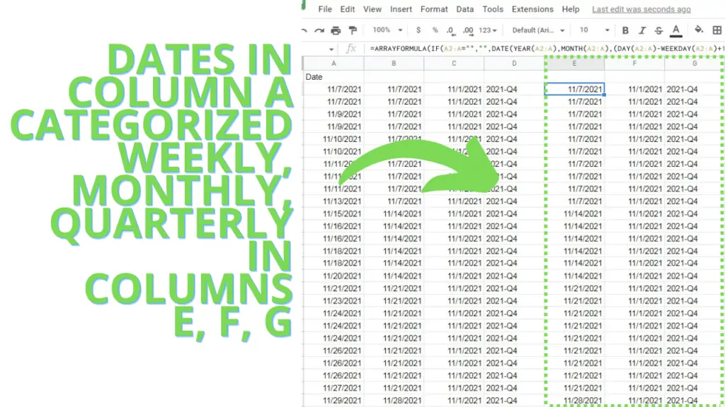
You can test the array formulas by adding new dates after the last entry on column A. You will notice that the columns on the right are populated with their corresponding date categories, without the need to add another new formula.
Frequently Asked Question in Adding Week, Month, and Quarter Categories to Dates in Google Sheets
Will the formulas in Google Sheets still work on dates of a different format?
Formulas in Google Sheets will work on dates in different formats. As long as Google Sheets recognizes the date, it should be stored as a datevalue, which the formulas can properly process.
Can I apply a different kind of date formatting to a formula that outputs a date in Google Sheets?
As long as a formula in Google Sheets outputs a date instead of a string of characters, you can choose a different date format for it through the Format Menu. An example is formatting mm-dd-yyyy dates to dd/mm/yyyy dates. For the rest, either switch to using a formula that outputs a date and then format the result into a different date, or apply a custom text formatting to a formula that outputs a text.
Conclusion on Adding Date Categories in Google Sheets
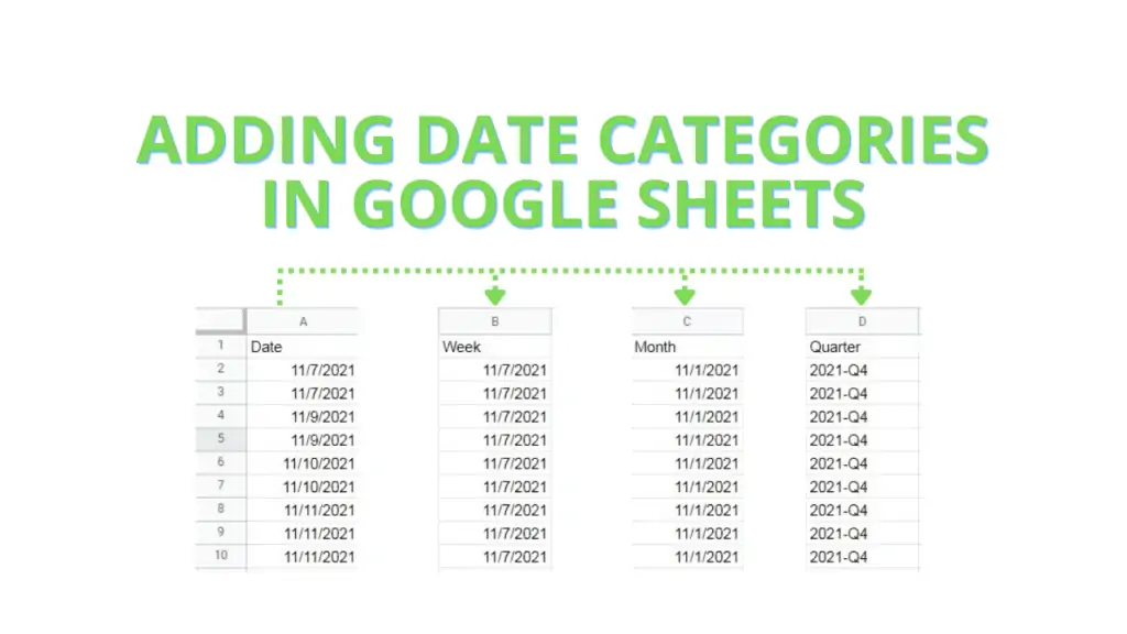
To add date categories in Google Sheets prepare the dates that you want to categorize. It’s best to store all of the dates in a single, continuous line.
For all of the formulas, simply substitute all instances of [date] with the cell address of the date you want to categorize.
Next, apply the weekly category formula
“=DATE(YEAR([date]),MONTH([date]),(DAY([date])-WEEKDAY([date])+[week start]))”
to the right of your dates column.
Next, apply the monthly category formula
“=DATE(YEAR([date]),MONTH([date]),1)”
to the right of your weekly category column.
Finally, apply the quarterly category formula
“=YEAR([date])&”-“&”Q”&ROUNDUP(MONTH([date])/3)”
to the right of your monthly category column.

