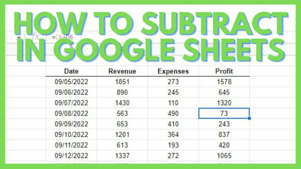
In this tutorial, I am going to discuss how to subtract in Google Sheets.
Even if a calculator may help you solve most if not all mathematical problems, once you need to subtract thousands of numbers it is better to work with spreadsheets. In this tutorial, I am going to show you how to best subtract in Google Sheets.
How to Subtract in Google Sheets
- Select a cell and enter edit mode
- Type in “=” and enter the first number (minuend)
- Add “-” and enter the second number (subtrahend)
- Hit enter

Subtraction in Google Sheets Video Tutorial (Step-By-Step)
2 Ways to Subtract in Google Sheets
It’s easy to subtract in Google Sheets and there are 2 ways that you can do this. I’ve listed them below.
1. Using the Minus Symbol (-)
The most straightforward way to subtract in Google Sheets is by using the Minus Symbol or Operator which is represented by a dash (-).
The syntax for this is:
=Value1-Value2
Value1 is referred to as the minuend, which is the number to be subtracted from. While Value2 is the subtrahend, the number is to be taken from Value1.
In the example below is a report for NPS (Net Promoter Scores) taken from an analysis of survey results. It is computed by subtracting the percentage of the negative scores from the positive ones. Applying the syntax to this example, I got:
=(C3-D3)*100
Which is the difference between Positive-Negative multiplied by 100.
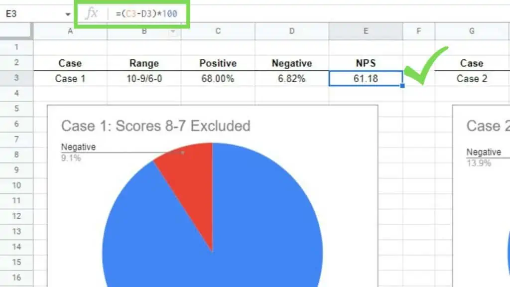
The parenthesis in this formula makes sure that the subtraction takes place first before anything else can be applied to the values, which would be wrong.
2. Using the MINUS Function
Another method to subtract in Google Sheets is by using the MINUS Function.
The syntax for MINUS is
=MINUS(Value1,Value2)
Similar to using the Minus operator, with the MINUS Function Value1 is referred to as the minuend as well and Value2 is the subtrahend. This cannot be interchanged, otherwise, the difference may be wrong.
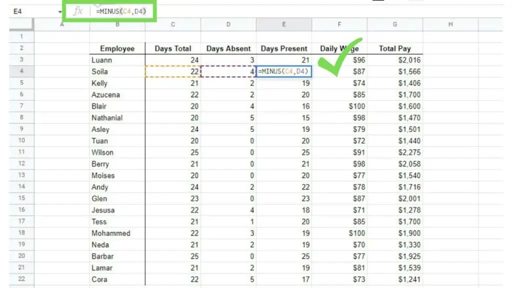
In the example below, I have a table showing a computation for the total pay of a certain group of employees. To do this, I had to know how many days were they present during this pay period. Applying the syntax below, I got:
=MINUS(C4,D4)
Which is the difference of (Days Total – Days Absent) applied to all the rows available.
In doing this, I was able to get the number of days each employee was present, multiply it by their daily wage, and know their total pay.
There is no difference between the results of the MINUS Function over the Minus operator (-) when both are used properly. Although the former can be easier to use while the latter can be more versatile depending on some situations.
3 Examples of How to Subtract in Google Sheets
Let’s look at 3 examples of how to subtract in Google Sheets using the Minus symbol or operator (-).
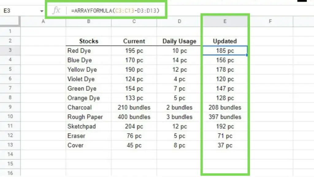
1. Using ARRAYFORMULA on Big Data
Big data is often associated with spreadsheets. Using Google Sheets you can apply subtraction to multiple rows or columns in one go.
And this is where the ARRAYFORMULA Function comes in.
The difference here is that instead of subtracting one value from the other, we just need to adjust it with the ARRAYFORMULA in mind.
=ARRAYFORMULA(value1_range – value2_range)
An important thing is that both value ranges must have the same number of rows or columns. For reference, see my example below.
ARRAYFORMULA is a powerful function that even works with dynamic datasets such as the results of the SORT Function.
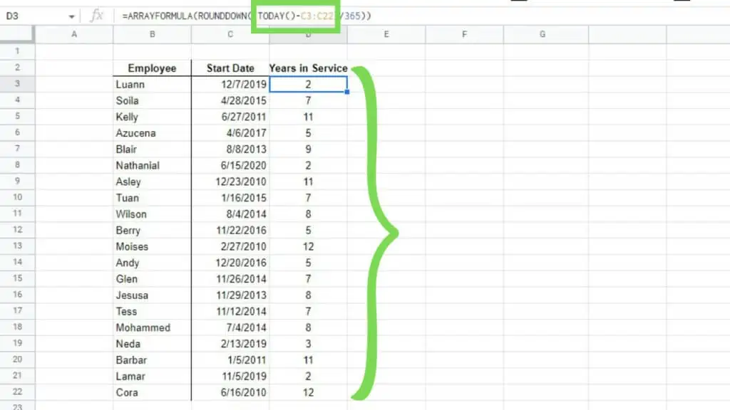
2. Using the TODAY Function for Dates
Another great benefit of using subtraction in Google Sheets is that you can also use it to manipulate dates.
This can be done easily with date functions such as TODAY.
In the example below, I used the Minus operator to get the difference between TODAY and each employee’s start date.
In doing so, I got the actual number of days as a difference. That in turn is divided by ‘365’, which is the total number of days in a year.
The ROUNDDOWN Function is simply used to get the actual year. The ARRAYFORMULA is then used to apply the entire formula to the whole dataset.
3. Using Values From Another Sheet or Workbook
It’s also possible to use interconnected databases across sheets or even workbooks. You may also be working on an “overview” sheet that will summarize data in different sheets and workbooks.
It’s similar to reference data from other sheets.
You just need to get the ‘sheet name’ and append an exclamation point (!) and then put in the cell or range address that you wish to reference.
Now, if you’re referencing from an entirely different workbook, you need to use the IMPORTRANGE Function instead. Its syntax is
=IMPORTRANGE(spreadsheet_url, range_string)
Where the spreadsheet_url is the actual URL of the file that you are referencing enclosed in double quotes.
While range_string is written similarly to when you’re just referencing other sheets in the same workbook (instructions above) which is also enclosed in double quotes.
See the example below where I used both.
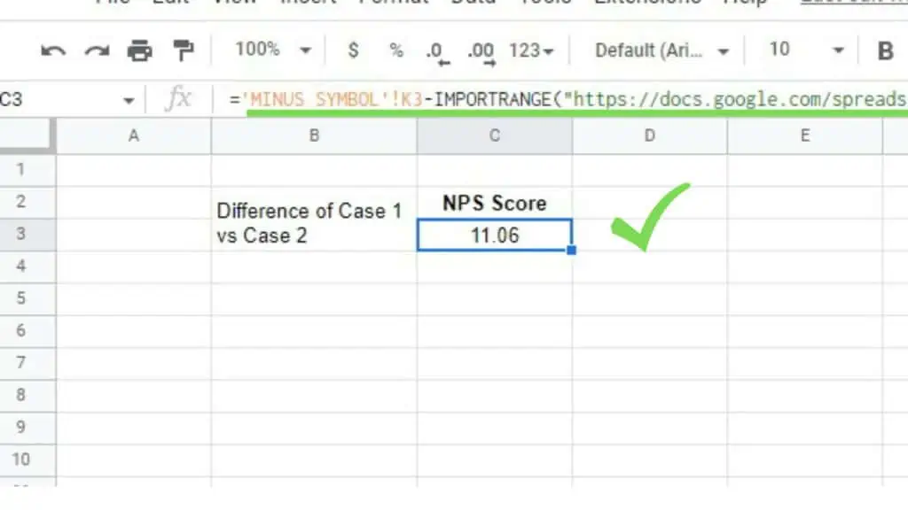
The formula for the example above is:
=’MINUS SYMBOL’!K3 – IMPORTRANGE(file_url,”MINUS SYMBOL!E3″)
I’ve presented the examples above separately but from my experience, the best way to subtract in Google Sheets is by combining several applications in one outcome.
Doing it this way will lead to more meaningful results.
Frequently Asked Questions about How to Subtract in Google Sheets
Can the two values of the MINUS Function be interchanged when I subtract in Google Sheets?
When you subtract in Google Sheets using the MINUS Function, the first value will always act as the minuend while the second one will be the subtrahend. The minuend is the number to be subtracted from therefore, these two values cannot be interchanged.
How can I subtract in Google Sheets other than using just the minus symbol or the MINUS Function?
You can also subtract in Google Sheets by using the SUM Function and having one of the values that will act as the subtrahend having a negative value. This will force SUM to conduct a subtraction instead of an addition.
Conclusion on How to Subtract in Google Sheets
You can subtract in Google Sheets by selecting a cell and entering edit mode. Then type in an equal sign “=” and enter the first number (minuend). Add the minus symbol or dash “-” and enter the second number (subtrahend). Finally, hit enter.

